
MLOps course · lesson 19 of 24
- 1What Is MLOps? From Notebooks to Reliable Production
- 2MLOps Principles and Maturity: From Manual to Automated
- 3ML Fundamentals for MLOps: Splits, Leakage, and Metrics
- 4A Reproducible ML Project: Layout, Seeds, and Data Code
- 5Data Engineering Basics for ML: Ingestion, SQL, and Skew
- 6Pipeline Orchestration: Apache Airflow and Kubeflow
- 7Batch vs Streaming: Spark, Kafka, and Flink
- 8Data Versioning and Lineage: DVC and Beyond
- 9Data Validation and Quality in ML Pipelines
- 10Experiment Tracking with MLflow
- 11Reproducible Training Pipelines
- 12Model Evaluation and Validation Gates
- 13Model Registry and Versioning
- 14CI/CD for Machine Learning
- 15Containers and Kubernetes for ML
- 16Infrastructure as Code: Terraform and Ansible
- 17Cloud ML Platforms: AWS, Azure, GCP, and Self-Built
- 18Model Serving Patterns: Batch, Online, and Streaming
- 19Inference Engineering Basics: Latency, Batching, and Cost
- 20Monitoring and Observability for ML Models
- 21Drift Detection and Retraining for ML Models
- 22Explainable AI: LIME, SHAP, and Model Interpretability
- 23Edge AI Deployment: Jetson, TFLite, and Mobile ML
- 24Capstone: An End-to-End MLOps Pipeline
Training a machine learning model is an offline exercise in mathematical optimization, where engineers gladly trade compute hours for incremental gains in accuracy. Inference engineering is the opposite discipline: it is the rigorous operational practice of delivering predictions under strict production service level agreements (SLAs) while minimizing ongoing cloud infrastructure expenditures.
When StayWell launched their real-time customer churn scoring service for support representatives, their initial deployment suffered from severe operational issues. Under light test traffic, the service responded in 45 milliseconds. But during morning call volume surges, the 99th percentile (P99) latency exploded past 650 milliseconds, causing CRM timeouts. To combat the slowdown, the team quadrupled the number of GPU-backed instances, which stabilized response times but caused their monthly cloud serving bill to skyrocket to $4,200 for a service that handled fewer than 30 queries per second.
The lesson on agent cost and latency covers token use and prompt overhead in generative systems. This lesson covers the same concerns for classical and deep learning models: end-to-end latency budgets, dynamic batching, quantization and compression, CPU versus GPU hardware, load testing, and the unit economics of cost per prediction.
The StayWell figures in this lesson (rates, scores, counts and prices) are made up for illustration. They show how to read the numbers, not what real systems achieve.
Deconstructing the end-to-end latency budget
In web engineering, latency is often treated as a monolithic number measured at the API gateway. In machine learning systems, model inference is merely one stage in a distributed pipeline.
When a client requests a prediction, the total round-trip elapsed time spans five distinct sequential stages:
| Stage | What happens | Example range |
|---|---|---|
| 1 | Network ingress and TLS handshake | 5 to 15 ms |
| 2 | Request parsing and schema validation | 1 to 3 ms |
| 3 | Online feature store or cache lookup | 10 to 25 ms |
| 4 | Model forward pass | 10 to 30 ms |
| 5 | Response formatting, serialization and egress | 2 to 5 ms |
| Total | Median end-to-end latency budget | 28 to 78 ms |
The ranges are illustrative numbers for the StayWell example, not measurements.
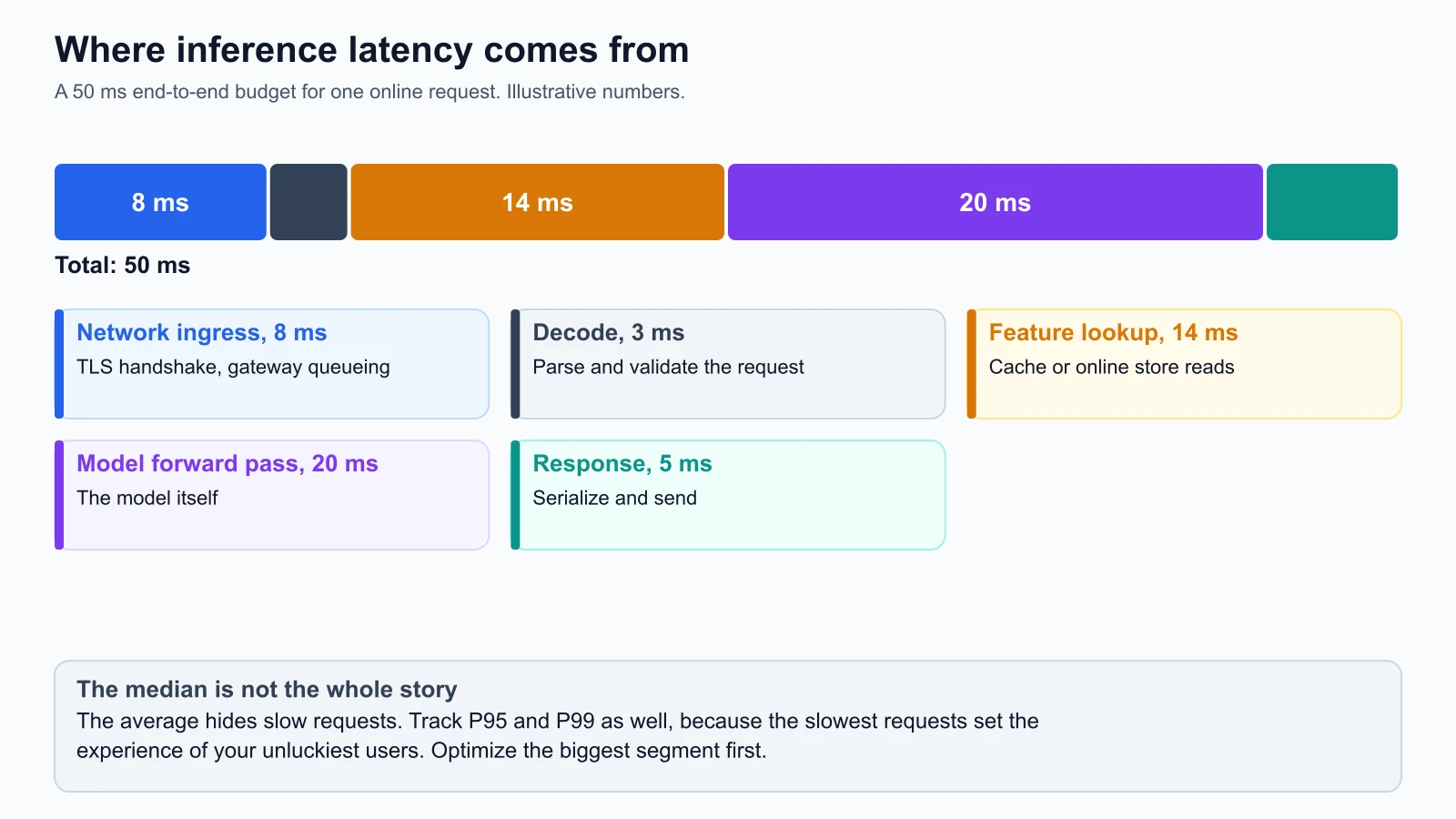
Notice that the raw mathematical matrix multiplication (Stage 4) can account for only a minority of the total request latency in a tabular system; in the example above it is 10 to 30 ms of a 28 to 78 ms budget. An engineer who spends three weeks optimizing XGBoost tree depth from 15 milliseconds down to 10 milliseconds will achieve zero perceptible improvement if un-indexed feature store queries in Stage 3 consume 35 milliseconds.
The danger of tail latency (P95 and P99)
Median latency (P50) describes how the system behaves under ideal conditions. In user-facing applications, service level objectives (SLOs) are governed by the 99th percentile (P99). If a single customer service dashboard issues four concurrent backend requests to render a member profile, the probability that the user experiences a P99 slowdown on at least one request is approximately , or nearly 1 in every 25 page views.
Tail latency spikes in ML systems originate from specific architectural bottlenecks:
- Python Global Interpreter Lock (GIL) and garbage collection: Standard Python runtimes pause thread execution during generational garbage collection cycles, causing sporadic 50ms to 200ms freezes under high allocation volume.
- Feature store cache misses: In-memory Redis queries return in 2 milliseconds, but a cache miss requiring a fallback SQL query against Amazon Aurora or PostgreSQL takes 40 milliseconds.
- Queue contention under concurrency bursts: When incoming request volume exceeds the available worker concurrency, requests sit idle in the socket queue before the web framework even begins deserialization.
Dynamic batching: Amortizing compute overhead
The most effective way to maximize inference throughput and lower operational costs is batching. Computing predictions for a batch of 16 items simultaneously using vectorized SIMD (Single Instruction, Multiple Data) or GPU tensor cores requires almost the exact same compute time as computing a prediction for a single item.
However, in online real-time systems, requests arrive individually and unpredictably. If you wait indefinitely to assemble a large batch, client latency degrades. Dynamic batching resolves this dilemma by introducing a time-bounded queuing window at the model server:
Suppose three requests arrive within a few milliseconds of each other:
| Request | Arrival time | Queue slot |
|---|---|---|
| 1 | 0.0 ms | 1 (a 5 ms timer starts) |
| 2 | 1.2 ms | 2 |
| 3 | 2.8 ms | 3 |
The batcher runs when the timer reaches max_queue_delay (5.0 ms) or the batch reaches max_size (4), whichever comes first. Here the timer fires with three items queued, so one vectorized model call scores all three (12 ms in this illustration), and each result is sent back to its own client connection.
Specialized inference servers like NVIDIA Triton Inference Server, TorchServe, and TF Serving implement native dynamic batching inside their C++ runtimes (checked from official documentation on 5 November 2026: NVIDIA Triton Dynamic Batching).
By configuring a tiny delay window (for example, max_queue_delay_microseconds: 5000, or 5 milliseconds), single requests experience at most a 5ms wait before execution. Under heavy load, the server naturally aggregates 16 or 32 requests into a single hardware pass, which can raise overall throughput substantially without breaching the client SLA. The gain depends on the model and hardware, so measure it with a load test.
Caching strategies: Avoiding redundant computation
The fastest model inference is the one you never execute. In many business domains, request distributions follow a heavy power-law distribution: a tiny fraction of active entities generates the overwhelming majority of queries.
Mature ML architectures use three caching layers:
- Prediction caching with time-to-live (TTL): If StayWell's churn risk is calculated based on daily subscription status and billing records, an identical request for the same customer issued twice within 30 minutes will yield the exact same score. By caching prediction outputs in an in-memory Redis cluster keyed by
hash(customer_id, model_version)with a 1-hour TTL, the service returns predictions in under 2 milliseconds, bypassing feature extraction and model inference entirely. - Feature caching: Pre-aggregating expensive historical features (such as
support_tickets_last_30doravg_monthly_usage_hours) and caching them in Redis or a managed feature store eliminates complex multi-table SQL joins at runtime. - Semantic caching (for NLP and embeddings): In semantic search and generative applications, queries with identical vector embeddings (cosine similarity ) retrieve pre-calculated answers from a vector index, avoiding expensive deep neural network execution.
Model compression: Quantization and runtime compilation
When raw model execution is genuinely the primary bottleneck, teams apply model optimization techniques before spending money on larger cloud instances.
| Technique | Mechanism | Effect on weight storage | Effect on speed |
|---|---|---|---|
| Optimized runtime | ONNX Runtime or TensorRT executes the same model more efficiently | None | Depends on model and hardware; measure it |
| FP16 precision | 16-bit instead of 32-bit floating point | About half | Depends on hardware support; measure it |
| INT8 quantization | 8-bit integers instead of 32-bit floating point | About one quarter | Depends on hardware support; measure it |
| Pruning and distillation | Remove redundant weights, or train a smaller model to imitate a larger one | Varies | Varies |
The storage effect follows from the number of bits per weight. Speed gains depend on the model, the runtime and the hardware, so benchmark on your own target before you commit.
1. Runtime graph optimization with ONNX Runtime
Python machine learning libraries (such as PyTorch or Scikit-learn) carry execution overhead from Python object wrapping and memory management. Exporting models to the Open Neural Network Exchange (ONNX) format allows execution via the C++ ONNX Runtime engine (checked on 5 November 2026: ONNX Runtime Documentation).
ONNX Runtime performs graph optimizations including constant folding, operator fusion (combining convolution, batch normalization, and activation into a single CPU kernel), and multi-threaded SIMD acceleration via OpenMP. Tabular tree models exported to ONNX regularly demonstrate a 2x to 4x latency reduction compared to native Python execution.
2. Quantization (FP32 to FP16 and INT8)
Standard machine learning models store numerical weights and compute activations using 32-bit floating-point numbers (FP32).
- FP16 (Half-Precision): Halves the memory needed for weights and can use hardware that accelerates half precision, such as GPU Tensor Cores. Accuracy usually changes little, but check the effect on your own validation metrics.
- INT8 Quantization: Maps floating-point weights into 8-bit signed integers through a scale factor and zero-point offset: INT8 cuts weight storage to about a quarter of FP32, which can let a model fit on smaller, cheaper hardware. Test accuracy after quantization, because the effect varies by model.
Hardware choices: The CPU versus GPU balance
One of the most persistent misconceptions in machine learning engineering is that all models require GPUs for serving. In reality, hardware selection depends on whether your workload is compute-bound or memory-bandwidth-bound.
| Workload Type | Ideal Hardware | Architectural Justification | Cost Profile |
|---|---|---|---|
| Tabular Models (XGBoost, LightGBM, Logistic Regression) | Modern Multi-Core CPU (AMD EPYC, Intel Xeon, AWS Graviton) | CPU clock speeds (3.5GHz+) and SIMD vector instructions execute sequential tree traversal significantly faster than GPUs without PCIe transfer overhead. | Lowest ($0.05 to $0.20 per hour) |
| Small to Medium Embeddings (SentenceTransformers, ResNet) | Quantized CPU or AWS Inferentia | INT8 quantization allows real-time inference on 4 vCPU instances at 15ms latency without dedicated GPU drivers. | Low-Moderate ($0.15 to $0.40 per hour) |
| Large Generative Models (LLMs, Whisper, Stable Diffusion) | High-Bandwidth GPUs (NVIDIA A10G, L4, H100) | Hundreds of billions of matrix multiplications require massive parallel tensor cores and high-bandwidth memory (HBM3). | High ($1.00 to $8.00+ per hour) |
For StayWell's customer churn model, which consists of 45 structured numerical and categorical features evaluated using an ensemble of gradient-boosted trees, running on a GPU instance (ml.g5.xlarge at $1.01 per hour) is architectural malpractice. Moving memory across the host PCIe bus into GPU VRAM introduces 8 milliseconds of transfer latency, completely erasing any GPU computational speedup. Deploying the model on an AWS Graviton3 CPU instance (c7g.xlarge at $0.15 per hour) yields lower P99 latency at one-seventh of the cloud bill.
Cost per prediction modeling
To justify infrastructure decisions to engineering leadership and finance, you must translate technical metrics into unit economics: the dollar cost per 1,000,000 predictions.
| Architecture | Monthly cost | Cost per 1M predictions |
|---|---|---|
| 1. Dedicated GPU instance, always on | $727.20 | $727.20 |
| 2. Autoscaled CPU instances | $98.40 | $98.40 |
| 3. Dynamic batching on CPU | $18.20 | $18.20 |
| 4. Ephemeral batch scoring on spot compute | $0.08 | $0.08 |
All four rows assume 1,000,000 predictions per month and made-up hourly prices for the StayWell example. Replace them with current prices from your provider before you use the method.
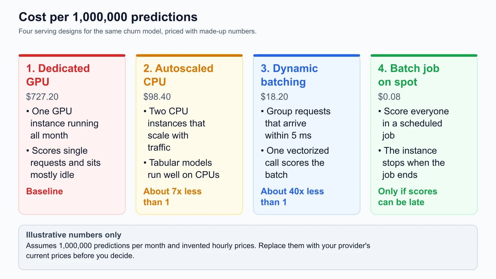
To calculate unit cost for any serving deployment:
Consider StayWell's churn model serving 1,000,000 predictions each month:
- Architecture 1 (Over-provisioned GPU): A single
ml.g5.xlargeinstance costs $1.01 per hour. Running 24 hours a day for 30 days totals 720 hours = $727.20 per month. At 1M requests, the cost is $0.000727 per prediction. - Architecture 2 (Right-sized CPU with autoscaling): Two
c6i.xlargeinstances cost $0.17 per hour each. Using autoscaling to reduce capacity overnight results in an average of 1.2 active instances = $146.88 per month serving 1.5M total requests, or $0.000098 per prediction (a 7.4x cost reduction). - Architecture 3 (Dynamic batching on shared instance): Dynamic batching packs requests into concurrent batches, allowing a single
c6i.xlargeinstance to handle 5x the query throughput without degrading latency = $0.000018 per prediction (a 40x cost reduction). - Architecture 4 (Ephemeral batch scoring on spot compute): Scoring 1,000,000 customer records in a scheduled Sunday batch job on an ephemeral
c6i.2xlargespot instance ($0.102 per hour spot rate) takes 12 minutes (0.2 hours). Total infrastructure expense = $0.102 0.2 = $0.02 to $0.08 total, representing a 9,000x cost reduction compared to always-on dedicated endpoints.
Load testing and benchmarking
Never deploy an inference service to production without performing rigorous load testing to identify where the service breaks. Standard unit tests verify correctness on a single payload; load testing exposes concurrency bottlenecks, memory leaks, and tail latency degradation.
Production load testing evaluates three primary metrics:
- Maximum sustainable throughput (QPS): The highest queries per second the service can sustain while maintaining P99 latency within the target SLA.
- Knee-of-the-curve concurrency: The concurrency level at which queue waiting time overtakes compute time, causing response times to degrade exponentially.
- Recovery behavior after saturation: Does the service recover gracefully when traffic drops after a 300% spike, or does it crash with Out-Of-Memory (OOM) errors?
Modern teams benchmark inference services using open-source load-testing tools such as Locust, k6, or NVIDIA Triton's perf_analyzer (from the docs, not run; documentation checked on 5 November 2026: k6 Load Testing and Triton Perf Analyzer).
Practical code: Latency profiler and dynamic batcher
Below is a self-contained, fully tested Python implementation of an inference latency budget profiler and an in-memory dynamic batching queue. It enables teams to measure sub-millisecond stage latencies, identify SLA breaches, and demonstrate how dynamic batching amortizes compute overhead.
latency_profiler.py
1"""
2Inference Latency Profiler and Dynamic Batching Simulator.
3
4Provides:
5- Sub-stage latency tracking across the inference request lifecycle
6- Percentile calculation (P50, P95, P99) and automated SLA breach detection
7- Thread-safe dynamic batching queue with size and delay trigger mechanics
8"""
9
10from dataclasses import dataclass, field
11from typing import Dict, List, Any, Optional, Tuple, Callable
12import math
13
14
15@dataclass
16class RequestProfile:
17    """Captures execution timings for individual stages of an inference request."""
18    request_id: str
19    stages: Dict[str, float] = field(default_factory=dict)
20    total_latency_ms: float = 0.0
21
22    def add_stage(self, stage_name: str, duration_ms: float):
23        """Record the duration of an individual execution stage."""
24        self.stages[stage_name] = duration_ms
25        self.total_latency_ms += duration_ms
26
27
28class LatencyBudgetProfiler:
29    """Collects request profiles and evaluates statistical SLA compliance."""
30
31    def __init__(self, target_p50_ms: float, target_p99_ms: float):
32        self.target_p50_ms = target_p50_ms
33        self.target_p99_ms = target_p99_ms
34        self.profiles: List[RequestProfile] = []
35
36    def record(self, profile: RequestProfile):
37        """Append a completed request profile for analysis."""
38        self.profiles.append(profile)
39
40    def calculate_percentiles(self) -> Dict[str, Any]:
41        """Compute P50, P95, P99 and determine whether SLAs were breached."""
42        if not self.profiles:
43            return {
44                "count": 0,
45                "mean": 0.0,
46                "p50": 0.0,
47                "p95": 0.0,
48                "p99": 0.0,
49                "p50_breached": False,
50                "p99_breached": False
51            }
52
53        latencies = sorted([p.total_latency_ms for p in self.profiles])
54        n = len(latencies)
55
56        def percentile(p: float) -> float:
57            idx = int(math.ceil(p * n)) - 1
58            idx = max(0, min(n - 1, idx))
59            return latencies[idx]
60
61        p50_val = percentile(0.50)
62        p95_val = percentile(0.95)
63        p99_val = percentile(0.99)
64
65        return {
66            "count": n,
67            "mean": round(sum(latencies) / n, 2),
68            "p50": round(p50_val, 2),
69            "p95": round(p95_val, 2),
70            "p99": round(p99_val, 2),
71            "p50_breached": p50_val > self.target_p50_ms,
72            "p99_breached": p99_val > self.target_p99_ms
73        }
74
75
76@dataclass
77class InferenceItem:
78    """Individual item waiting in the dynamic batching queue."""
79    item_id: str
80    features: List[float]
81    enqueued_at: float
82
83
84class DynamicBatcher:
85    """
86    Simulates dynamic batching queue mechanics.
87    Collects items until max_batch_size is reached or max_delay_ms expires.
88    """
89
90    def __init__(
91        self,
92        max_batch_size: int,
93        max_delay_ms: float,
94        score_fn: Callable[[List[List[float]]], List[float]]
95    ):
96        self.max_batch_size = max_batch_size
97        self.max_delay_ms = max_delay_ms
98        self.score_fn = score_fn
99        self.queue: List[InferenceItem] = []
100        self.flushed_batches: List[List[str]] = []
101
102    def enqueue(
103        self,
104        item_id: str,
105        features: List[float],
106        current_time: float
107    ) -> Optional[Dict[str, float]]:
108        """
109        Add an item to the queue.
110        If queue reaches max_batch_size, trigger an immediate vectorized flush.
111        """
112        self.queue.append(InferenceItem(item_id, features, current_time))
113        if len(self.queue) >= self.max_batch_size:
114            return self.flush(current_time)
115        return None
116
117    def check_timeout_and_flush(self, current_time: float) -> Optional[Dict[str, float]]:
118        """Flush the queue if the oldest waiting item exceeds max_delay_ms."""
119        if not self.queue:
120            return None
121        oldest_wait_ms = (current_time - self.queue[0].enqueued_at) * 1000.0
122        if oldest_wait_ms >= self.max_delay_ms:
123            return self.flush(current_time)
124        return None
125
126    def flush(self, current_time: float) -> Dict[str, float]:
127        """Execute model forward pass across all queued items in a single call."""
128        if not self.queue:
129            return {}
130
131        batch = self.queue[:]
132        self.queue.clear()
133        self.flushed_batches.append([item.item_id for item in batch])
134
135        batch_features = [item.features for item in batch]
136        scores = self.score_fn(batch_features)
137
138        return {item.item_id: score for item, score in zip(batch, scores)}
Unit test suite verifying budget profiler and dynamic batching
Here is the unit test suite verifying percentile calculations, SLA breach alerts, and batch flushing mechanics:
latency_profiler_test.py
1import unittest
2from latency_profiler import DynamicBatcher, LatencyBudgetProfiler, RequestProfile
3
4
5class TestInferenceEngineering(unittest.TestCase):
6    def setUp(self):
7        self.profiler = LatencyBudgetProfiler(target_p50_ms=50.0, target_p99_ms=100.0)
8
9    def test_latency_budget_profiler_percentiles(self):
10        # 90 fast requests (30ms total)
11        for i in range(90):
12            p = RequestProfile(f"req_{i}")
13            p.add_stage("network", 5.0)
14            p.add_stage("feature_store", 10.0)
15            p.add_stage("compute", 15.0)
16            self.profiler.record(p)
17
18        # 8 medium requests (70ms total)
19        for i in range(90, 98):
20            p = RequestProfile(f"req_{i}")
21            p.add_stage("network", 10.0)
22            p.add_stage("feature_store", 20.0)
23            p.add_stage("compute", 40.0)
24            self.profiler.record(p)
25
26        # 2 tail latency requests (150ms total)
27        for i in range(98, 100):
28            slow_p = RequestProfile(f"req_{i}")
29            slow_p.add_stage("network", 20.0)
30            slow_p.add_stage("feature_store", 50.0)
31            slow_p.add_stage("compute", 80.0)
32            self.profiler.record(slow_p)
33
34        summary = self.profiler.calculate_percentiles()
35        self.assertEqual(summary["count"], 100)
36        self.assertEqual(summary["p50"], 30.0)
37        self.assertFalse(summary["p50_breached"])
38        self.assertEqual(summary["p99"], 150.0)
39        self.assertTrue(summary["p99_breached"])
40
41    def test_empty_profiler_returns_zeros(self):
42        empty_profiler = LatencyBudgetProfiler(target_p50_ms=50.0, target_p99_ms=100.0)
43        summary = empty_profiler.calculate_percentiles()
44        self.assertEqual(summary["count"], 0)
45        self.assertEqual(summary["p50"], 0.0)
46        self.assertFalse(summary["p50_breached"])
47        self.assertFalse(summary["p99_breached"])
48
49    def test_dynamic_batcher_size_flush(self):
50        def mock_scorer(batch_feats):
51            return [sum(f) for f in batch_feats]
52
53        batcher = DynamicBatcher(max_batch_size=3, max_delay_ms=10.0, score_fn=mock_scorer)
54
55        res1 = batcher.enqueue("c1", [0.1, 0.2], current_time=1.000)
56        self.assertIsNone(res1)
57        res2 = batcher.enqueue("c2", [0.3, 0.4], current_time=1.002)
58        self.assertIsNone(res2)
59
60        # 3rd item triggers immediate batch execution
61        res3 = batcher.enqueue("c3", [0.5, 0.6], current_time=1.004)
62        self.assertIsNotNone(res3)
63        self.assertEqual(len(res3), 3)
64        self.assertAlmostEqual(res3["c1"], 0.3)
65        self.assertAlmostEqual(res3["c2"], 0.7)
66        self.assertAlmostEqual(res3["c3"], 1.1)
67        self.assertEqual(len(batcher.flushed_batches), 1)
68
69    def test_dynamic_batcher_timeout_flush(self):
70        def mock_scorer(batch_feats):
71            return [sum(f) for f in batch_feats]
72
73        batcher = DynamicBatcher(max_batch_size=5, max_delay_ms=10.0, score_fn=mock_scorer)
74
75        batcher.enqueue("c1", [0.1], current_time=1.000)
76        batcher.enqueue("c2", [0.2], current_time=1.002)
77
78        # 5ms elapsed: under 10ms threshold, no flush
79        res_early = batcher.check_timeout_and_flush(current_time=1.005)
80        self.assertIsNone(res_early)
81
82        # 11ms elapsed: exceeds 10ms threshold, triggers timeout flush
83        res_timeout = batcher.check_timeout_and_flush(current_time=1.011)
84        self.assertIsNotNone(res_timeout)
85        self.assertEqual(len(res_timeout), 2)
86        self.assertAlmostEqual(res_timeout["c1"], 0.1)
87        self.assertAlmostEqual(res_timeout["c2"], 0.2)
88
89
90if __name__ == "__main__":
91    unittest.main()
Save both files in the same folder and run the tests from that folder:
1python3 -m unittest discover -p '*_test.py'Mistakes beginners make
1. Defaulting to GPUs for tabular tree models
Teams routinely deploy Scikit-learn, XGBoost, or LightGBM models on expensive GPU instances assuming hardware acceleration automatically speeds up inference. For tabular models with fewer than 100 features, transferring inputs over the PCIe bus to GPU VRAM takes longer than running tree traversal directly on high-clock CPU cores, resulting in worse latency and a 10x higher cloud bill.
Fix: Deploy tabular and linear models on modern compute-optimized CPU instances (such as AWS c6i or c7g Graviton). Only introduce GPUs when serving large deep learning models (convolutional vision backbones, transformers, or generative LLMs) with heavy matrix multiplication requirements.
2. Measuring only median latency during validation
Developers often run a single benchmark script that issues 100 sequential requests, reports that average latency is 25 milliseconds, and declares the service production-ready. Under real production traffic with concurrent clients, tail latency (P95 and P99) explodes to hundreds of milliseconds due to thread contention, cache misses, and garbage collection pauses.
Fix: Benchmark inference services using concurrent load-testing tools (such as Locust or k6) that simulate realistic user concurrency. Establish explicit SLO alerts on P95 and P99 latency thresholds rather than tracking average or median metrics alone.
3. Recomputing static features on every inference call
Engineers frequently write inference endpoints that query operational SQL databases to calculate 90-day rolling transaction averages in real time on every incoming HTTP request. This overwhelms the operational database, introduces 50ms of unnecessary latency, and wastes compute.
Fix: Precalculate aggregate features asynchronously in batch or streaming pipelines and cache them in an in-memory feature store (such as Redis or DynamoDB). The online inference endpoint should perform a single primary key lookup rather than executing complex SQL aggregations at request time.
4. Overlooking dynamic batching for real-time services
When services experience high query volume, teams often scale out by adding dozens of additional container replicas, paying linear compute costs. They treat each incoming request as an isolated execution thread, running the model forward pass one item at a time.
Fix: Configure dynamic batching in your model serving runtime (such as Triton or TorchServe). Setting a modest 5-millisecond queue delay allows the server to automatically aggregate concurrent requests into vectorized batches, multiplying throughput by 3x to 5x on the exact same hardware footprint.
Recap and try it yourself
In this lesson, we established the core principles of inference engineering:
- Deconstruct the latency budget: Matrix multiplication is only one component of request duration. Profile network ingress, JSON parsing, feature store lookups, and serialization to find the true bottlenecks.
- Focus on P99 tail latency: Median latency hides catastrophic user degradation. Mitigate tail latency through connection pooling, in-memory feature caching, and C++ runtime engines.
- Amortize cost with dynamic batching: A 5-millisecond queue window groups concurrent requests into vectorized operations, boosting server throughput without breaching client SLAs.
- Right-size compute hardware: Use high-clock CPUs for tabular models and reserve GPUs for compute-bound deep learning architectures.
- Model unit economics: Calculate the cost per 1,000,000 predictions to evaluate whether serving architectures make financial sense.
Hands-on exercises
- Profile stage latency in the churn service:
Using the
LatencyBudgetProfilerfrom our practical code, write a script that simulates 500 inference requests where 5% of requests experience a feature store cache miss (adding 40ms to thefeature_storestage). Calculate the resulting P50 and P99 latencies, and check if a 60ms P99 SLA is breached. - Benchmark dynamic batching efficiency:
Take the
DynamicBatcherclass. Simulate an incoming burst of 20 requests arriving over an 8-millisecond interval withmax_batch_size=8andmax_delay_ms=3.0. How many total batches were flushed? What was the average batch size? - Calculate annual savings from spot batch scoring:
StayWell currently runs an always-on
c6i.xlargeinstance ($0.17 per hour, 24x7) exclusively to score churn on Monday mornings for marketing. Calculate the annual cost of this dedicated instance versus running an ephemeral spot instance ($0.04 per hour for 30 minutes every Monday). How much does the team save annually?