Batch vs Streaming: Spark, Kafka, and Flink

Most machine learning failures in production start with infrastructure choices that solve problems the team does not actually have. When an engineering team hears that real-time features improve churn prediction, the default reaction is often to deploy a Kafka cluster, set up Spark Structured Streaming or Apache Flink, and wire up an elaborate streaming mesh. Six months and thousands of dollars in cloud spend later, the team discovers that their data volume could have been processed in four seconds on a single laptop using DuckDB.

Real-time feature processing is genuine engineering with genuine trade-offs. It brings operational complexity, network partitions, state serialization overhead, out-of-order event management, and difficult backfill requirements. Building on what we covered in data engineering fundamentals and pipeline orchestration with Airflow and Kubeflow, you must understand how batch and streaming pipelines differ, how engines like Apache Spark, Apache Kafka, and Apache Flink work under the hood, and how to assess whether your problem demands distributed infrastructure.

In this lesson, we examine data processing paradigms for machine learning through the lens of StayWell. You will learn the mechanics of distributed batch processing, the distributed log abstraction, stateful stream processing, and a systematic framework for deciding what engine belongs in your stack.

Three modes of data processing for machine learning

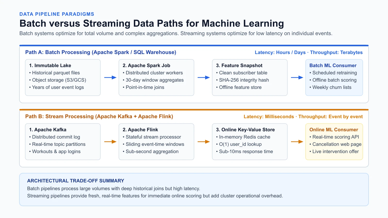
Data processing for machine learning falls into three architectural patterns: pure batch, micro-batch, and low-latency continuous streaming. Each pattern balances latency, throughput, implementation complexity, and operational cost differently.

Pure batch processing

Pure batch processing collects raw data over a fixed calendar interval, such as an hour, a day, or a month. Once the collection window closes, a compute engine spins up, reads the entire slice from durable storage, performs transformations, and writes the output dataset to disk or an analytical store.

Batch processing prioritizes throughput over latency. Because the engine processes large blocks of data at once, it optimizes disk reads through sequential scans, parallelizes work across CPU cores, and minimizes network handshake overhead. Batch jobs run on scheduled intervals managed by orchestrators like Airflow.

In the StayWell customer churn scenario, batch features describe long-term behavior patterns:

• Total room nights booked in the last twelve months
• Average cancellation rate across all lifetime reservations
• Net Promoter Score submitted during checkout sixty days ago
• Total revenue generated across all stays over two years

These metrics evolve slowly. Computing them every second provides zero predictive advantage over computing them once every midnight. If a customer stayed at a resort last month, their twelve-month reservation total does not change at 2:15 PM today unless they complete a new transaction. Running a daily batch job to refresh these aggregations is cost-efficient, reproducible, and simple to debug.

Micro-batch processing

Micro-batching bridges pure batch and continuous streaming. Rather than processing twenty-four hours of data at midnight, the engine collects incoming records in memory for a short window, typically between five hundred milliseconds and thirty seconds. It then dispatches that small collection through a standard batch execution engine.

Apache Spark Structured Streaming popularized this approach. The benefit of micro-batching is architectural reuse: you write your transformation logic using DataFrame transformations, and the engine executes the same plan whether reading a historical Parquet archive or a stream of five-second micro-batches.

Micro-batching works well when feature freshness requirements range from tens of seconds to a few minutes:

• Updating reservation counts per region every fifteen minutes
• Aggregating payment gateway error rates over five-minute sliding intervals
• Ingesting hotel review sentiment within thirty seconds of submission

The limitation of micro-batching is high-frequency latency. Because the engine waits for the collection window to elapse before running scheduling and execution passes, latencies below one hundred milliseconds are unattainable.

Low-latency continuous streaming

Continuous stream processing evaluates events record by record as they occur. There is no batching window on ingestion. As soon as a network socket receives an event, the processing thread executes transformations, updates internal state, and emits results to an egress queue.

Engines like Apache Flink adopt this continuous event-driven model. The trade-off is operational overhead. Continuous stream processors maintain long-running stateful services that run 24 hours a day, 7 days a week. Unlike batch jobs that release cloud instances after finishing, stream processing clusters consume compute resources continuously, requiring dedicated monitoring for memory fragmentation, backpressure, and checkpoint storage.

Continuous streaming is necessary only when the machine learning model must act within milliseconds of an action:

• Detecting fraudulent payment attempts before authorizing a transaction
• Adjusting dynamic room pricing while a guest refreshes their checkout cart
• Identifying a sudden cluster of session errors to trigger an immediate customer support prompt

Distributed batch processing with Apache Spark

When dataset sizes exceed the physical memory of a single computer, distributed computing frameworks distribute data partitions across a cluster of worker machines. Apache Spark is the standard open-source framework for distributed data processing.

The official Apache Spark Documentation (verified on 4 November 2026) describes Spark as a multi-language engine for executing data engineering, data science, and machine learning on single-node machines or clusters.

Core architecture: driver and executors

A running Spark application consists of a single Driver program and one or more Executor processes distributed across cluster nodes:

1. The Driver: The Driver process runs your application's main() function. It constructs the logical execution graph, converts it into a physical execution plan of stages and tasks, and coordinates work through a cluster manager (such as Kubernetes, YARN, or Spark's standalone cluster manager). The Driver does not process large datasets directly; it directs the orchestra.
2. The Executors: Executors are worker processes running on cluster nodes. Each executor runs individual tasks assigned by the Driver, keeps data partitions in memory or spills them to local disk, and returns execution metrics back to the Driver.

RDDs, DataFrames, and Catalyst optimization

Historically, Spark exposed Resilient Distributed Datasets (RDDs), which are immutable, partitioned collections of objects evaluated lazily. Modern Spark applications build on DataFrames and the Catalyst Optimizer:

• Lazy Evaluation: When you invoke transformations on a DataFrame (such as filter(), select(), or groupBy()), Spark does not immediately touch the underlying storage. Instead, it records these steps in a Directed Acyclic Graph of logical operators.
• The Catalyst Optimizer: When an action (such as write() or count()) triggers execution, the Catalyst optimizer analyzes the logical graph. It reorders operations, pushes filter conditions directly into the storage layer (predicate pushdown), eliminates unused columns, and compiles the plan into optimized Java bytecode.
• Data Partitions: DataFrames are divided into discrete physical chunks called partitions. Spark assigns one executor core to process one partition at a time. If a dataset has two hundred partitions, Spark can run up to two hundred tasks in parallel if sufficient cores are available.

The shuffle bottleneck

Distributed processing is fast only when tasks run independently on local partitions without exchanging data across the network (known as narrow transformations, such as map or filter).

When an operation requires grouping or joining data by a specific key across the entire cluster (such as groupBy("user_id") or joining two large tables), Spark must reorganize data so that all records with the same key reside on the same executor. This data movement is called a shuffle.

Shuffles write intermediate partitions to local disk, transfer gigabytes across physical network switches, and force receiving executors to sort and merge streams. Shuffles are the primary source of out-of-memory errors, disk spills, and slow jobs in Spark pipelines.

Here is an example of an Apache Spark batch job that computes customer loyalty metrics for StayWell:

1# Spark batch feature aggregation for StayWell loyalty metrics
2# Reference: Apache Spark SQL Documentation (from the docs, not run)
3from pyspark.sql import SparkSession
4from pyspark.sql import functions as F
5
6def compute_monthly_churn_features(input_path: str, output_path: str) -> None:
7    # Initialize SparkSession with optimized shuffle partitions
8    spark = SparkSession.builder \
9        .appName("StayWell-Monthly-Churn-Features") \
10        .config("spark.sql.shuffle.partitions", "200") \
11        .getOrCreate()
12
13    # Read historical bookings from partitioned Parquet storage
14    bookings_df = spark.read.parquet(input_path)
15
16    # Compute aggregate features grouped by customer
17    feature_df = bookings_df.groupBy("customer_id").agg(
18        F.count("booking_id").alias("total_lifetime_bookings"),
19        F.sum("total_usd").alias("total_lifetime_spend_usd"),
20        F.avg("total_usd").alias("avg_booking_value_usd"),
21        F.sum(F.when(F.col("status") == "CANCELLED", 1).otherwise(0)).alias("total_cancelled_bookings"),
22        F.max("checkout_date").alias("last_checkout_date")
23    ).withColumn(
24        "cancellation_rate",
25        F.col("total_cancelled_bookings") / F.col("total_lifetime_bookings")
26    )
27
28    # Write curated features back to analytical storage
29    feature_df.write \
30        .mode("overwrite") \
31        .parquet(output_path)
32
33    spark.stop()

Notice that this script calculates long-range historical features from raw transactional data. When your input dataset reaches hundreds of gigabytes or terabytes, Spark's partitioned execution handles the workload predictably.

The event backbone: Apache Kafka

Before any engine can process streaming features, a durable messaging backbone must ingest events from upstream web applications, point-of-sale systems, and mobile apps.

The official Apache Kafka Documentation (verified on 4 November 2026) defines Kafka as a distributed event streaming platform used for high-performance data pipelines, streaming analytics, and data integration.

The distributed commit log abstraction

Unlike traditional message queues (like RabbitMQ or ActiveMQ) that discard messages as soon as a worker acknowledges receipt, Kafka treats data streams as an append-only distributed commit log.

• Topics and Partitions: Events are published to named categories called topics. A topic is divided into one or more partitions. Each partition is an ordered, immutable sequence of records stored on disk across Kafka broker servers.
• Append-Only Writes: When a publisher writes an event, the broker appends it to the end of the partition and assigns it a sequential integer identifier called an offset.
• Log Retention: Kafka preserves records regardless of whether they have been read. Retention policies define how long records stay on disk (for example, seven days or until disk limits are reached). Multiple consumers can read the same records independently at their own pace.

Consumer groups and offsets

Consumers track their own reading progress through the topic by committing their current offset back to a special Kafka internal topic.

A Consumer Group consists of multiple consumer instances working cooperatively to read from a topic. Kafka assigns each partition within a topic to exactly one consumer in the group:

• If a topic has four partitions and your consumer group has four worker processes, each worker reads one partition in parallel.
• If a consumer crashes, Kafka rebalances partition assignments to the remaining live consumers.
• If a downstream feature pipeline experiences a bug, you can stop the consumer, deploy a code fix, reset the offset to an earlier timestamp, and replay historical events without data loss.

Backpressure and decoupled architectures

A critical virtue of Kafka for machine learning is backpressure decoupling. If your ML inference microservice or feature transformer slows down during peak shopping traffic, the upstream API servers do not crash waiting for responses. Upstream web servers append events to Kafka and return immediately. The slower downstream consumer processes the log as quickly as it can, absorbing traffic spikes safely.

Here is an example of an event publisher and a consumer configuration using Python:

1# Kafka event publisher for StayWell booking activity
2# Reference: Confluent Kafka Python Documentation (from the docs, not run)
3import json
4from confluent_kafka import Producer, Consumer
5
6# Configure the Kafka Producer for high-throughput durable delivery
7producer_conf = {
8    "bootstrap.servers": "kafka-broker1.internal:9092,kafka-broker2.internal:9092",
9    "client.id": "staywell-booking-api",
10    "acks": "all",  # Ensure all in-sync replicas acknowledge write
11    "compression.type": "snappy"
12}
13
14producer = Producer(producer_conf)
15
16def emit_booking_event(customer_id: str, booking_id: str, amount_usd: float) -> None:
17    payload = {
18        "event_type": "BOOKING_CREATED",
19        "customer_id": customer_id,
20        "booking_id": booking_id,
21        "amount_usd": amount_usd,
22        "timestamp_ms": 1730764800000
23    }
24    # Keying by customer_id guarantees all events for a customer land on the same partition
25    producer.produce(
26        topic="staywell.bookings.v1",
27        key=customer_id.encode("utf-8"),
28        value=json.dumps(payload).encode("utf-8")
29    )
30    producer.poll(0)

Partitioning by customer_id is essential for machine learning. It guarantees that all events relating to a single customer are processed in the strict chronological order they occurred.

Stateful stream processing with Apache Flink

Ingesting events through Kafka is only the first step. To use those events in machine learning, you must transform raw clicks, searches, and cancellations into aggregated feature values in real time. This requires stateful stream processing.

The official Apache Flink Documentation (verified on 4 November 2026) describes Flink as a framework and distributed processing engine for stateful computations over unbounded and bounded data streams.

Event time versus processing time

In real-world networks, the moment an event occurs is rarely the exact moment your stream processing engine receives it. A guest might search for hotel rooms on a mobile app in an airport, lose cell connectivity inside an elevator, and have their phone transmit the batch of search events five minutes later:

• Processing Time: The local clock time of the machine executing the stream transformation. Processing time is easy to use, but results are non-deterministic: replaying the same log tomorrow yields different aggregation windows because the wall-clock time differs.
• Event Time: The timestamp embedded inside the record when the action occurred on the client device. Event-time processing produces identical, reproducible features whether data arrives in real time or gets replayed during historical backfills.

Watermarks and out-of-order data

When using event time, how does the engine know when all events for a specific time window have arrived? It cannot wait forever for disconnected mobile devices.

Flink solves this with Watermarks. A watermark is a control record injected into the stream that carries a timestamp $T$. When an operator receives a watermark with timestamp $T$, it assumes that no subsequent events with a timestamp earlier than $T$ will arrive. Once the watermark passes the window's end time, the operator finalizes its calculation and emits the window result.

Window types: tumbling, sliding, and session

Feature engineering over continuous streams relies on temporal windows:

• Tumbling Windows: Fixed-size, non-overlapping intervals. For example, calculating total search queries in distinct five-minute blocks (00:00 to 00:05, 00:05 to 00:10).
• Sliding Windows: Fixed-size, overlapping intervals. For example, computing customer search volume over the last sixty minutes, evaluated every one minute. Each event belongs to multiple overlapping windows.
• Session Windows: Dynamic intervals bounded by periods of user inactivity. If a customer searches for rooms, browses photos, and checks reviews over twelve minutes, then stops for thirty minutes, Flink groups those actions into a single coherent session.

1// Apache Flink sliding window aggregation for real-time customer feature updates
2// Reference: Apache Flink Streaming API Documentation (from the docs, not run)
3DataStream<CustomerSearchEvent> searchStream = env
4    .addSource(new FlinkKafkaConsumer<>("staywell.searches.v1", new SearchEventSchema(), kafkaProps))
5    .assignTimestampsAndWatermarks(
6        WatermarkStrategy.<CustomerSearchEvent>forBoundedOutOfOrderness(Duration.ofSeconds(10))
7            .withTimestampAssigner((event, timestamp) -> event.getEventTimestamp())
8    );
9
10// Key by customer ID and calculate search frequency in a 15-minute sliding window
11DataStream<CustomerSearchFeature> searchFeatures = searchStream
12    .keyBy(CustomerSearchEvent::getCustomerId)
13    .window(SlidingEventTimeWindows.of(Time.minutes(15), Time.seconds(30)))
14    .aggregate(new SearchCountAggregator());

Flink maintains the internal state of open windows in high-performance storage (such as RocksDB) and periodically takes distributed snapshots called checkpoints to object storage. If a worker node crashes, Flink restores its internal state from the latest checkpoint, resumes the Kafka offsets, and continues processing without losing or duplicating data.

When you do not need distributed engines

Distributed systems come with heavy operational taxes:

• Distributed debugging requires aggregating log streams across dozens of virtual containers.
• Network serialization and deserialization eat significant CPU cycles.
• Upgrading cluster software requires orchestrating rolling restarts and verifying schema registries.
• Small datasets processed on distributed engines often run slower than on a single laptop due to task scheduling and coordination overhead.

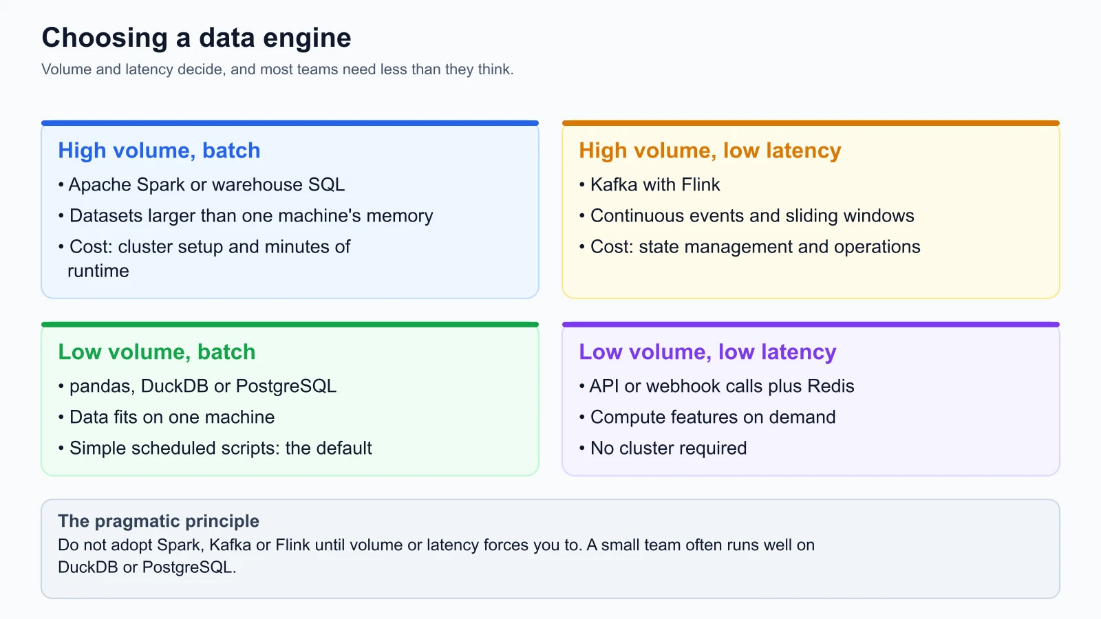
Before adopting Spark, Kafka, or Flink, consider the single-node modern alternatives.

The modern single-node stack: DuckDB and Polars

Modern single-node hardware is extraordinarily capable. Cloud providers routinely offer virtual instances with 128 virtual CPUs and 512 gigabytes of RAM. A single server of that size can process tens of millions of records in seconds.

The official DuckDB Documentation (verified on 4 November 2026) highlights its columnar vectorized execution engine designed for high-performance analytical queries. DuckDB runs embedded inside your Python process, requires zero external daemon processes, and processes Parquet files directly from disk without loading entire datasets into memory.

Similarly, the Polars Documentation (verified on 4 November 2026) demonstrates how Rust-powered multi-threaded columnar DataFrames execute complex transformations with a fraction of the memory footprint of traditional libraries.

A clear decision framework

Use this decision checklist when architecting data pipelines for machine learning:

1. Volume check: Does your raw dataset fit within the memory or NVMe storage of a single large cloud server (under 1 terabyte)? If yes, start with DuckDB or Polars. You will achieve faster iteration cycles, instant CI test runs, and minimal maintenance costs.
2. Batch scale check: Does your historical dataset exceed several terabytes, requiring horizontal scaling across dozens of nodes, or does it integrate directly with enterprise data lakes managed by cloud platforms? If yes, adopt Apache Spark.
3. Latency check: Does your model require feature updates within sub-second intervals to make a live prediction? If no, use scheduled batch runs. If yes, deploy Kafka as your event log and Flink (or Spark Structured Streaming) for stream processing.

Real-world case study: StayWell online feature ingestion

To see how these concepts fit together, let us examine StayWell's customer churn architecture.

The StayWell requirements

StayWell wants to identify customers at risk of churning while they are browsing the web portal. The churn scoring service evaluates two distinct categories of features:

1. Batch historical features:

• Account tenure in months
• Total number of completed stays in the last 24 months
• Historical cancellation percentage
• Average review rating submitted by the guest

2. Streaming dynamic features:

• Search frequency during the current browsing session (last 15 minutes)
• Number of checkout errors encountered in the last 30 minutes
• Whether the customer visited the cancellation policy FAQ in the last hour

The hybrid feature architecture

Rather than forcing all data through a streaming engine, StayWell implements a two-path design:

• Path 1: Nightly batch pipeline. An Airflow DAG triggers an Apache Spark job (or DuckDB script during early stages) at 02:00 UTC. The job reads all completed booking records from the data lake, computes lifetime metrics, and writes the resulting feature values into an analytical feature table and an online key-value store (such as Redis or Amazon DynamoDB).
• Path 2: Real-time event pipeline. When a user browses the website, the web application emits user actions to an Apache Kafka topic keyed by customer_id. A lightweight stream processing job reads from Kafka, computes rolling counts across sliding windows, and continuously updates the dynamic feature keys in the same Redis store.
• Inference time: When the customer loads their account page, the churn prediction service fetches both the precomputed batch features and the streaming session features by querying Redis using the customer_id. It combines both vectors into a single feature array and invokes the churn classification model in under twenty milliseconds.

This hybrid pattern delivers the best of both worlds: complex historical aggregations are calculated efficiently in batch, while high-velocity session signals update in real time without straining the database.

Mistakes beginners make

1. Adopting Kafka and Flink for batch-friendly problems

Engineers often assume that building a real-time streaming pipeline makes their architecture superior. They spend weeks deploying Kafka clusters, managing Zookeeper or KRaft metadata, and configuring stream watermarks for features that only need updating once a day.

Fix: Start every feature pipeline as a scheduled batch job. Only migrate a feature to a streaming pipeline when an A/B test or explicit business requirement proves that sub-minute feature freshness directly improves model prediction quality.

2. Overlooking partition keys in Kafka

Publishing messages to Kafka without defining a message key causes the broker to distribute events round-robin across partitions. If events for the same customer land on different partitions, downstream stream processors cannot guarantee chronological processing order, corrupting time-series features.

Fix: Always assign a deterministic entity key, such as customer_id, to every event published to Kafka. All events for that specific entity will route to the same partition, guaranteeing strict chronological sequence.

3. Ignoring the cost of Spark shuffles

Beginner Spark developers write chained groupBy(), distinct(), and join() operations without considering physical partition layouts. When massive datasets shuffle across physical cluster networks, executors run out of memory, jobs spill data to disk, and cloud bills surge.

Fix: Filter and project your data as early as possible in the transformation pipeline. Use broadcast joins when joining large tables against small lookup tables (broadcast(small_df)), avoiding unnecessary full-cluster data shuffles.

4. Relying on processing time instead of event time

Developers frequently use the current system clock when computing streaming window features. When network interruptions occur or when historical data is replayed during model retraining, processing-time aggregations produce completely different results than what actually occurred in the user's session.

Fix: Always embed an event timestamp in the record payload at generation time. Configure your streaming framework to use event-time semantics with bounded out-of-order watermarks to ensure deterministic feature calculation during both real-time ingestion and historical backfilling.

Recap and try it yourself

In this lesson, you explored the operational and architectural trade-offs between batch and streaming systems:

• Pure batch processing maximizes throughput and cost-efficiency for slowly changing metrics.
• Distributed batch engines like Apache Spark scale out horizontally through driver-executor hierarchies and the Catalyst optimizer, but require careful management of shuffle operations.
• Apache Kafka acts as an append-only distributed commit log, enabling decoupled architectures, replayability, and consumer group scalability.
• Apache Flink provides true continuous stream processing with event-time semantics, watermarks, and stateful sliding window aggregations.
• Single-node analytical engines like DuckDB and Polars often outperform distributed clusters on datasets under one terabyte without operational overhead.

Try it yourself

To practice comparing batch and streaming concepts hands-on, implement this diagnostic experiment on your local machine:

1. Simulate event logs: Write a Python script using standard library modules (json, time, random) that generates one thousand booking and search events for fifty unique customers and writes them to a local JSON Lines file.
2. Compute tumbling window features: Write a pure Python function that reads the JSON Lines file and computes the number of searches per customer in five-minute event-time tumbling windows. Handle out-of-order records by sorting events by their embedded timestamp before window assignment.
3. Benchmark against DuckDB: If you have DuckDB installed locally, write an analytical SQL query that computes the same rolling customer search metrics directly from the JSON file using DuckDB's window functions. Compare the execution speed and code simplicity between the custom loop and the vectorized SQL query.