
MLOps course · lesson 3 of 24
- 1What Is MLOps? From Notebooks to Reliable Production
- 2MLOps Principles and Maturity: From Manual to Automated
- 3ML Fundamentals for MLOps: Splits, Leakage, and Metrics
- 4A Reproducible ML Project: Layout, Seeds, and Data Code
- 5Data Engineering Basics for ML: Ingestion, SQL, and Skew
- 6Pipeline Orchestration: Apache Airflow and Kubeflow
- 7Batch vs Streaming: Spark, Kafka, and Flink
- 8Data Versioning and Lineage: DVC and Beyond
- 9Data Validation and Quality in ML Pipelines
- 10Experiment Tracking with MLflow
- 11Reproducible Training Pipelines
- 12Model Evaluation and Validation Gates
- 13Model Registry and Versioning
- 14CI/CD for Machine Learning
- 15Containers and Kubernetes for ML
- 16Infrastructure as Code: Terraform and Ansible
- 17Cloud ML Platforms: AWS, Azure, GCP, and Self-Built
- 18Model Serving Patterns: Batch, Online, and Streaming
- 19Inference Engineering Basics: Latency, Batching, and Cost
- 20Monitoring and Observability for ML Models
- 21Drift Detection and Retraining for ML Models
- 22Explainable AI: LIME, SHAP, and Model Interpretability
- 23Edge AI Deployment: Jetson, TFLite, and Mobile ML
- 24Capstone: An End-to-End MLOps Pipeline
In the previous lessons on what MLOps is and MLOps principles and maturity levels, we explored the software systems and governance practices required to operate models in production. However, to design dependable pipelines and evaluation gates, an engineer must speak the model builder's language.
You do not need a research degree in mathematical statistics to build production MLOps systems. You do, however, need a firm grasp of how models learn from data, why data partitioning matters, where data leakage corrupts pipelines, and how to evaluate predictions against real business tradeoffs.
In this lesson, you will learn the core machine learning concepts that directly shape operations: supervised learning pipelines, clean data splitting, leakage vectors, classification metrics, overfitting, and framework trade-offs. You will also see how these concepts apply directly to StayWell, our running customer churn case study.
Supervised learning: features, labels, and algorithms
Most operational machine learning systems in industry use supervised learning. In supervised learning, an algorithm learns a mathematical mapping from input variables to a known target output based on historical examples.
Supervised learning systems work with two primary concepts:
- Features (): The measurable properties or attributes of the entity being analyzed. In StayWell's customer churn system, features include account tenure in months, weekly workout sessions completed, coach chat messages sent, and billing failure counts.
- Target or label (): The outcome the model attempts to predict. For StayWell, the target is binary: if the subscriber cancels their membership within the next thirty days, or if they remain active.
The goal of the algorithm (such as a logistic regression or decision tree) is to discover a mathematical function that predicts such that the difference between the prediction and the real label is minimized across unseen data.
In production, models encounter two broad categories of supervised tasks:
- Classification: Predicting a discrete category, such as whether an email is spam, whether a transaction is fraudulent, or whether a subscriber will churn.
- Regression: Predicting a continuous numeric value, such as predicting customer lifetime value in dollars or server CPU utilization thirty minutes into the future.
Data partitioning: train, validation, and test sets
The most common failure in machine learning engineering is evaluating a model on the same data used to train it. If an algorithm memorizes historical training records, it can achieve a perfect score while failing completely on fresh production requests.
To measure real generalization performance, you must partition available data into three strictly separated sets:
| Set | Typical share | Purpose |
|---|---|---|
| Training | about 70% | Optimization algorithms fit the model weights. |
| Validation | about 15% | Engineers tune hyperparameters and compare competing models. |
| Test | about 15% | Held back for the final release check before deployment. |
- Training set (typically 60% to 80%): The data exposed directly to the model's optimization algorithm. The algorithm adjusts internal weights and decision thresholds using these examples.
- Validation set (typically 10% to 20%): An independent dataset used during experimentation. Engineers evaluate model checkpoints on the validation set to tune hyperparameters (such as tree depth or regularization penalties) and select the champion algorithm.
- Test set (typically 10% to 20%): A quarantined dataset held in reserve until the end of development. The test set simulates production: it is evaluated only once to verify that the selected champion model has not overfit the validation set.
Random splits versus time-based splits
In academic datasets, partitioning is often performed using uniform random sampling (train_test_split). In production MLOps, random splitting is frequently an operational mistake.
When records represent customer behavior over time, events exhibit temporal dependency. If you train on records from Wednesday, validate on records from Tuesday, and test on records from Monday, your model learns patterns using information from the future.
For chronological event data like StayWell's subscriber activity, you must use time-based splits (also called out-of-time validation). You train on records from January through June, validate on July, and test on August. This forces the model to predict forward in time, exactly as it must in production.
Data leakage: how invalid signals enter pipelines
Data leakage occurs when information from outside the training dataset contaminates the model during training, giving the model access to signals that will not exist when making predictions in live production.
Leakage creates a deceptive failure mode: the model achieves stellar evaluation metrics in development, but fails immediately upon deployment.
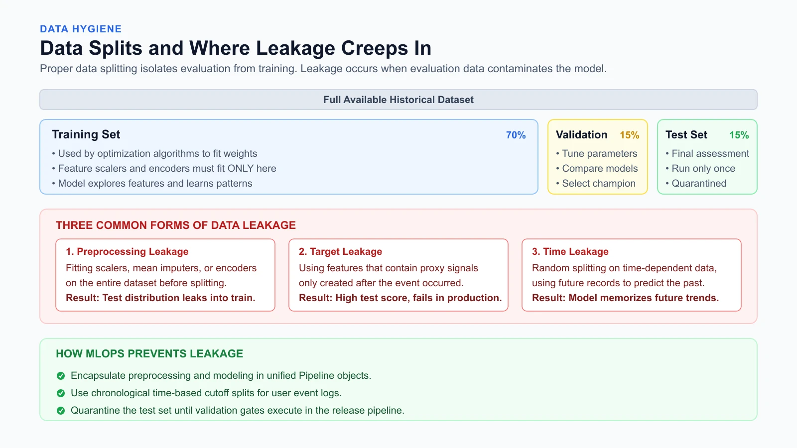
As visualized above, leakage enters pipelines through three primary vectors:
1. Preprocessing leakage
Preprocessing leakage happens when data transformations (such as scaling numeric values or imputing missing numbers with the column mean) are calculated across the entire dataset before splitting.
If you compute the mean of an input feature across all historical records and use it to replace missing values, the training set now contains statistical knowledge about the test set.
The rule: All scalers, encoders, and imputers must calculate parameters strictly on the training partition (fit). Those learned parameters are then applied without modification to the validation and test sets (transform).
2. Target leakage
Target leakage occurs when an input feature incorporates information that is only created after or concurrently with the target event.
Consider StayWell's churn prediction model. Suppose a database table includes a column called cancellation_survey_reason or account_status_updated_timestamp. If an engineer includes this column as a training feature, the model will learn that having a survey response predicts churn with near-perfect accuracy. In production, however, a user only completes a cancellation survey after they decide to leave, rendering the model useless for proactive intervention.
3. Time leakage
Time leakage happens when models use future events to predict past events due to improper temporal splitting. For instance, computing a rolling 30-day average workout count that includes workouts logged after the prediction cutoff date exposes the model to future facts.
Preventing leakage with scikit-learn pipelines
In Python, the most dependable way to eliminate preprocessing leakage is to encapsulate transformations and estimators inside a scikit-learn Pipeline object:
1from sklearn.pipeline import Pipeline
2from sklearn.preprocessing import StandardScaler
3from sklearn.impute import SimpleImputer
4from sklearn.linear_model import LogisticRegression
5
6# Good practice: transformations fit only on training folds
7churn_pipeline = Pipeline([
8    ("imputer", SimpleImputer(strategy="median")),
9    ("scaler", StandardScaler()),
10    ("classifier", LogisticRegression(random_state=42))
11])
12
13# Calling fit() computes median and scale parameters ONLY on X_train
14churn_pipeline.fit(X_train, y_train)
15
16# Calling predict() applies the already-fitted parameters to X_test
17predictions = churn_pipeline.predict(X_test)
Because the Pipeline manages transformations internally, test records cannot contaminate training calculations.
Overfitting and underfitting
A central challenge in machine learning is balancing bias and variance:
- Underfitting (high bias): The model is too simple to capture the underlying structure in the data. An underfit model performs poorly on both the training set and the validation set. For example, using a simple straight line to predict a complex non-linear relationship results in underfitting.
- Overfitting (high variance): The model is too complex and memorizes random noise and idiosyncrasies in the training set rather than learning generalizable patterns. An overfit model achieves near-perfect scores on training data, but performance drops sharply on validation data.
1Model Complexity:   Low -------------------- Optimal -------------------- High
2Training Error:     High ------------------- Low ----------------------- Near Zero
3Validation Error:   High ------------------- Low ----------------------- High
4Condition:          Underfitting (High Bias) Generalizing               Overfitting (High Variance)
In MLOps, validation gates compare training metrics against validation metrics. If a training score is 98% while the validation score is 74%, the model is overfitting, and the automated pipeline should reject the candidate artifact.
Classification metrics and baselines
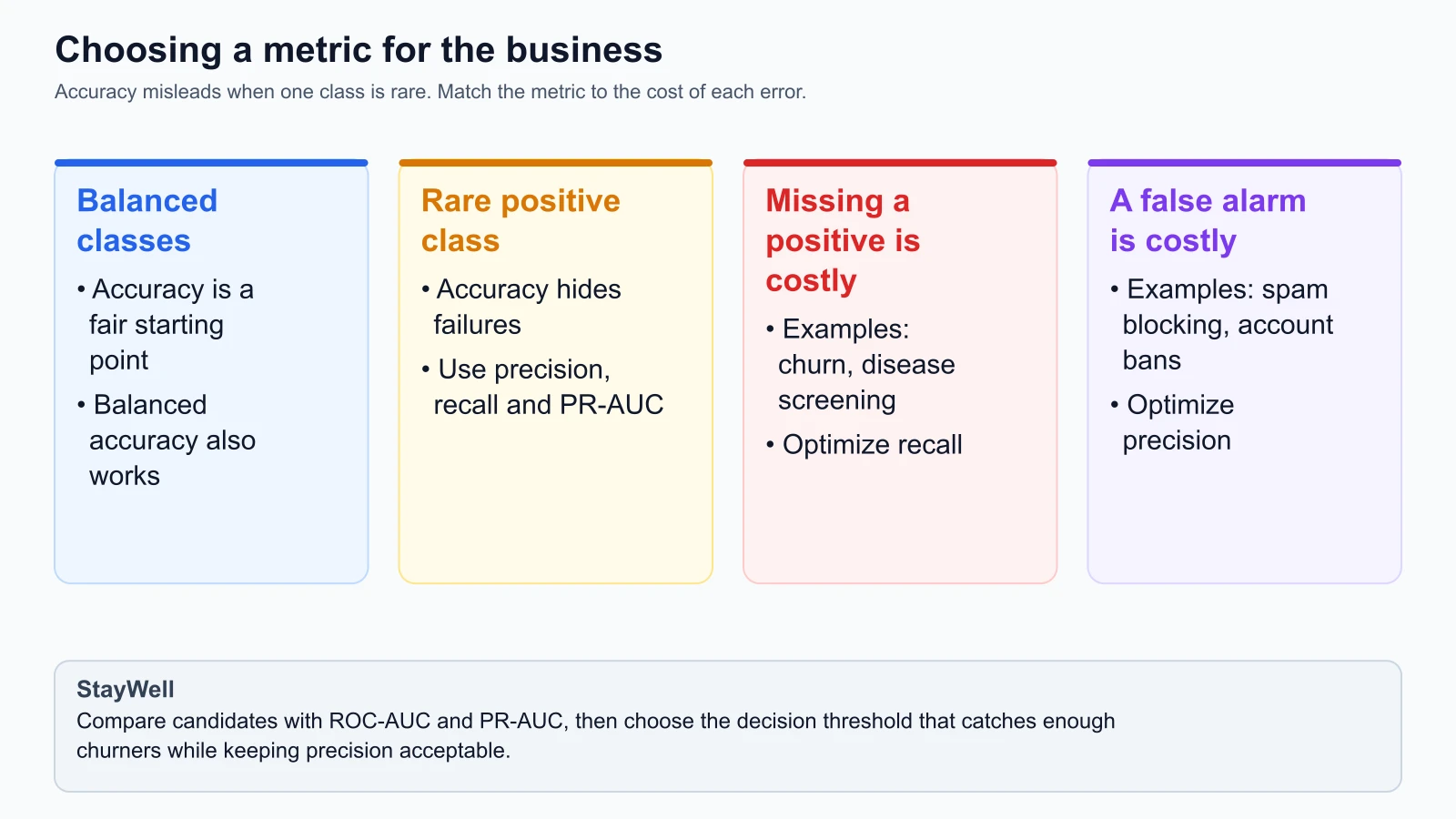
Evaluating a model requires selecting metrics that reflect business costs. Relying solely on global accuracy is one of the most common mistakes in machine learning.
Consider StayWell: in any given month, only 5% of active subscribers cancel their membership, while 95% stay. A naive baseline script that simply predicts "nobody will churn" for every customer achieves 95% accuracy without learning anything. Global accuracy is misleading when classes are imbalanced.
To evaluate predictions honestly, we use the confusion matrix:
| Actually Churned () | Actually Stayed () | |
|---|---|---|
| Predicted Churn () | True Positive (TP) | False Positive (FP) |
| Predicted Stay () | False Negative (FN) | True Negative (TN) |
From these four quadrants, we calculate domain-specific metrics:
Precision
Precision measures accuracy among positive predictions: out of all users the model flagged as churn risks, what proportion actually cancelled?
Optimize for precision when the cost of a false alarm (False Positive) is high. For example, in fraud detection, freezing an innocent user's bank account creates anger and support overhead. High precision ensures flagged accounts are genuinely fraudulent.
Recall (Sensitivity)
Recall measures completeness: out of all users who actually cancelled, what proportion did the model catch?
Optimize for recall when the cost of missing an event (False Negative) is high. In medical diagnostics or StayWell's subscriber retention, missing a customer who is about to churn means permanently losing subscriber revenue. A false alarm merely results in sending a check-in message or workout tip.
F1-Score
The F1-score is the harmonic mean of precision and recall. It provides a single summary score that balances both concerns:
Area Under the ROC Curve (ROC-AUC)
Most classifiers output a probability score between 0.0 and 1.0 rather than a hard category. A decision threshold (commonly 0.5 by default) converts this probability into a binary decision.
The Receiver Operating Characteristic (ROC) curve plots the True Positive Rate against the False Positive Rate across every possible decision threshold from 0.0 to 1.0.
The Area Under the Curve (ROC-AUC) quantifies how well the model separates positive and negative classes across all thresholds:
- : Perfect class separation.
- : No better than flipping a fair coin.
ROC-AUC is valuable for MLOps validation gates because it evaluates the model's fundamental ranking ability independent of the specific threshold chosen for production deployment.
Baseline comparisons
Before celebrating a model with an 84% ROC-AUC, an engineer must compare it against established baselines:
- Trivial baseline: A dummy model that predicts the majority class or outputs random guesses based on class prevalence.
- Simple heuristic baseline: A simple domain rule, such as "flag any user who logged zero workouts in the last fourteen days."
If an automated pipeline trains a complex gradient boosted ensemble that only performs marginally better than a two-line SQL heuristic, the engineering complexity and maintenance cost of serving the model may not be justified.
What deep learning changes for operations
While classic machine learning works on tabular datasets using algorithms like linear models and gradient boosted trees, deep learning uses multi-layered neural networks to learn representations from unstructured data such as text, images, and audio.
From an MLOps perspective, deep learning changes operational requirements:
- Hardware dependencies: Training deep learning models requires specialized accelerators (GPUs or TPUs). MLOps pipelines must manage driver installations (such as CUDA) and allocate GPU clusters dynamically.
- Training duration: While tabular models train in seconds or minutes on a standard CPU, deep learning models can train for hours, days, or weeks. Pipelines require checkpointing to resume training after hardware interruptions.
- Artifact dimensions: Tabular models like scikit-learn pipelines produce serialized files measured in megabytes. Deep learning model checkpoints often exceed several gigabytes, requiring specialized artifact storage and optimized container packaging.
- Explainability: Tabular models offer straightforward feature importance metrics. Deep neural networks operate as complex black-box functions, making debugging and compliance reporting more challenging.
Frameworks at a glance
Modern machine learning relies on distinct open-source frameworks depending on the problem domain:
| Framework | Primary domain | Common operational strengths |
|---|---|---|
| scikit-learn | Tabular data, classical ML (regression, trees, clustering) | Lightweight CPU execution, fast training, standardized pipeline APIs |
| PyTorch | Deep learning, research, computer vision, natural language | Dynamic execution graph, clean Pythonic debugging, dominant in modern research |
| TensorFlow / Keras | Deep learning, mobile deployment, embedded systems | Static graph optimization, mature export formats (SavedModel, TFLite) |
In this course, our hands-on tooling and StayWell case study focus on scikit-learn and tabular data. Tabular data accounts for the vast majority of operational predictive models in enterprise settings (churn prediction, credit scoring, lead qualification, and inventory forecasting).
Practical worked example: building a clean training script
To see these principles in code, here is an illustrative, self-contained Python script demonstrating a clean training workflow with data splitting, pipeline encapsulation, baseline comparison, and metric evaluation:
1import numpy as np
2from sklearn.datasets import make_classification
3from sklearn.model_selection import train_test_split
4from sklearn.pipeline import Pipeline
5from sklearn.preprocessing import StandardScaler
6from sklearn.linear_model import LogisticRegression
7from sklearn.dummy import DummyClassifier
8from sklearn.metrics import classification_report, roc_auc_score
9
10def run_experiment():
11    # 1. Generate synthetic binary classification dataset (StayWell churn proxy)
12    X, y = make_classification(
13        n_samples=2000,
14        n_features=10,
15        n_informative=6,
16        weights=[0.85, 0.15], # 15% churn rate (imbalanced)
17        random_state=42
18    )
19
20    # 2. Strict partitioning: 70% train, 15% validation, 15% test
21    X_train, X_temp, y_train, y_temp = train_test_split(
22        X, y, test_size=0.30, random_state=42, stratify=y
23    )
24    X_val, X_test, y_val, y_test = train_test_split(
25        X_temp, y_temp, test_size=0.50, random_state=42, stratify=y_temp
26    )
27
28    # 3. Establish baseline using dummy classifier (predicts most frequent class)
29    baseline = DummyClassifier(strategy="most_frequent")
30    baseline.fit(X_train, y_train)
31    baseline_acc = baseline.score(X_val, y_val)
32    print(f"Majority Baseline Accuracy: {baseline_acc:.3f}")
33
34    # 4. Construct leak-free pipeline
35    model_pipeline = Pipeline([
36        ("scaler", StandardScaler()),
37        ("classifier", LogisticRegression(random_state=42))
38    ])
39
40    # 5. Fit pipeline strictly on training data
41    model_pipeline.fit(X_train, y_train)
42
43    # 6. Evaluate on validation set
44    val_probs = model_pipeline.predict_proba(X_val)[:, 1]
45    val_preds = model_pipeline.predict(X_val)
46
47    val_auc = roc_auc_score(y_val, val_probs)
48    print(f"Validation ROC-AUC: {val_auc:.3f}")
49    print("\nValidation Classification Report:")
50    print(classification_report(y_val, val_preds, target_names=["Stay", "Churn"]))
51
52    # 7. Final test evaluation (executed once on champion model)
53    test_probs = model_pipeline.predict_proba(X_test)[:, 1]
54    test_auc = roc_auc_score(y_test, test_probs)
55    print(f"Final Quarantined Test ROC-AUC: {test_auc:.3f}")
56
57if __name__ == "__main__":
58    run_experiment()
Running this script with Python 3.12, NumPy 2.5.4 and scikit-learn 1.9.1 prints the output below. The exact digits can differ slightly on other library versions.
1Majority Baseline Accuracy: 0.850
2Validation ROC-AUC: 0.920
3
4Validation Classification Report:
5              precision    recall  f1-score   support
6
7        Stay       0.93      0.98      0.96       255
8       Churn       0.87      0.60      0.71        45
9
10    accuracy                           0.93       300
11   macro avg       0.90      0.79      0.83       300
12weighted avg       0.92      0.93      0.92       300
13
14Final Quarantined Test ROC-AUC: 0.917
The report shows why accuracy alone misleads. Overall accuracy is 93%, only eight points above the 85% a script gets by predicting that nobody churns. The churn row tells the real story: when the model flags a member as a churn risk it is right 87% of the time (precision), but it finds only 60% of the members who actually leave (recall). In later lessons you will tune the decision threshold so StayWell catches more churn risks before members leave.
The synthetic data comes from make_classification, so these numbers describe this exercise, not a real churn problem.
Pointers for mathematics and statistics
If you want to deepen your mathematical foundation for modeling, focus on three specific areas:
- Linear algebra: Vectors, matrices, dot products, and matrix multiplication underpin how features are represented and transformed computationally.
- Calculus: Partial derivatives and gradients power gradient descent, the optimization method used to train neural networks and linear models.
- Probability and statistics: Probability distributions, hypothesis testing, Bayes' theorem, and variance analysis inform data drift detection and evaluation metrics.
For MLOps practitioners, understanding how these concepts apply to operational error detection and data distribution shifts is far more valuable than solving textbook equations by hand.
Sources
Checked on 4 November 2026:
- Scikit-learn Documentation, Common pitfalls and recommended practices (Data Leakage).
- Scikit-learn API Reference, sklearn.pipeline.Pipeline.
- Google Machine Learning Crash Course, Classification: Precision and Recall.
Mistakes beginners make
When handling machine learning data and model validation, teams commonly make several errors:
1. Preprocessing data before the split
Developers often apply normalizers, scalers, or categorical encoders to an entire CSV file before splitting into train and test sets. This leaks future distribution statistics into the training fold, yielding artificially optimistic evaluation scores that fail in production.
Fix: Split your raw data first. Fit all transformers and scalers strictly on the training partition, or wrap your preprocessing and estimator inside a scikit-learn Pipeline.
2. Relying on random splits for time-series data
Using uniform random splitting on customer transactions, log records, or sensor readings leaks future temporal signals into the past. Models learn to interpolate between past and future points rather than forecasting ahead.
Fix: Use temporal cutoffs for time-dependent datasets. Train on past periods and evaluate on subsequent chronological periods to mirror production reality.
3. Tuning hyperparameters directly on the test set
When developers iteratively tweak model settings to improve scores on the test set, the test set becomes contaminated by human selection bias. The reported score no longer represents unbiased generalization.
Fix: Maintain a three-way split (train, validation, test). Tune hyperparameters exclusively on the validation set, and evaluate the quarantined test set only once as an operational gate.
4. Over-optimizing accuracy on imbalanced datasets
In fraud, defect detection, or customer churn, the positive class represents a small fraction of records. A model can achieve 99% accuracy by predicting negative for every sample while missing every single fraud event.
Fix: Select metrics that reflect the operational cost of errors, such as Precision, Recall, F1-Score, and PR-AUC. Always evaluate candidate models against a naive baseline.
Recap and try it yourself
In this lesson, you covered the machine learning fundamentals that anchor MLOps:
- Supervised learning maps input features () to known targets () through classification or regression.
- Honest evaluation requires partitioning data into training, validation, and quarantined test sets, using time-based splits for chronological event data.
- Data leakage occurs through preprocessing, target leakage, and time leakage, inflating development metrics while causing production failure.
- Scikit-learn pipelines encapsulate feature transformations and model fitting, preventing test set statistics from contaminating training.
- Classification metrics like Precision, Recall, and ROC-AUC evaluate business tradeoffs far more accurately than global accuracy on imbalanced datasets.
Try it yourself
To reinforce these concepts, work through these exercises:
- Spot the leakage: Suppose you are building a model to predict whether a loan application will default. Your dataset includes a feature called
debt_collection_agency_contact_count. Does this feature represent target leakage? Why or why not? - Select a metric for StayWell: If StayWell's marketing team has budget to call only one hundred high-risk subscribers each week, but wants to be confident that every called subscriber is genuinely likely to cancel, should you tune the model for high Precision or high Recall?
- Write a pipeline assertion: In the worked scikit-learn code example above, modify the pipeline to include a feature scaler. Verify that calling
churn_pipeline.named_steps["scaler"].mean_only reflects statistics fromX_train.
In the next lesson, we will set up a reproducible machine learning project layout, configure pinned dependencies, and build StayWell's synthetic data generator in Python.