
MLOps course · lesson 22 of 24
- 1What Is MLOps? From Notebooks to Reliable Production
- 2MLOps Principles and Maturity: From Manual to Automated
- 3ML Fundamentals for MLOps: Splits, Leakage, and Metrics
- 4A Reproducible ML Project: Layout, Seeds, and Data Code
- 5Data Engineering Basics for ML: Ingestion, SQL, and Skew
- 6Pipeline Orchestration: Apache Airflow and Kubeflow
- 7Batch vs Streaming: Spark, Kafka, and Flink
- 8Data Versioning and Lineage: DVC and Beyond
- 9Data Validation and Quality in ML Pipelines
- 10Experiment Tracking with MLflow
- 11Reproducible Training Pipelines
- 12Model Evaluation and Validation Gates
- 13Model Registry and Versioning
- 14CI/CD for Machine Learning
- 15Containers and Kubernetes for ML
- 16Infrastructure as Code: Terraform and Ansible
- 17Cloud ML Platforms: AWS, Azure, GCP, and Self-Built
- 18Model Serving Patterns: Batch, Online, and Streaming
- 19Inference Engineering Basics: Latency, Batching, and Cost
- 20Monitoring and Observability for ML Models
- 21Drift Detection and Retraining for ML Models
- 22Explainable AI: LIME, SHAP, and Model Interpretability
- 23Edge AI Deployment: Jetson, TFLite, and Mobile ML
- 24Capstone: An End-to-End MLOps Pipeline
Modern machine learning models, from gradient-boosted decision trees to deep neural networks, are frequently described as impenetrable black boxes. A model ingests dozens or hundreds of raw input features, executes millions of non-linear mathematical operations across high-dimensional tensor spaces, and outputs a single calibrated probability.
In academic benchmarks, high predictive accuracy is often the sole objective. In production engineering, a prediction without an explanation is an operational liability. When StayWell deployed their churn prediction model, customer service representatives were presented with a raw churn score: Customer #8812 has an 82% churn probability. When the customer called to complain about a billing discrepancy, the representative had no idea whether the model flagged the member because of their recent support tickets, high monthly charges, or expiring contract. To retain the member, the agent offered a $20 bill credit. The customer accepted the credit, yet cancelled their membership three days later because their technical app issues remained unresolved.
Had the representative seen an explanation revealing that support_tickets = 4 accounted for 60% of the risk while pricing was negligible, they would have routed the caller to an advanced technical specialist instead of offering a financial discount.
In Privacy, Bias, and Red Teaming, we analyzed safety and counterfactual evaluations in generative systems. In this lesson, we master Explainable AI (XAI) for MLOps. We differentiate between global and local interpretability, explore the mechanics of LIME and SHAP, break down what explanations can and cannot prove, conduct algorithmic fairness audits, establish reviewer documentation via Model Cards, and implement an additive feature attribution engine.
The StayWell figures in this lesson (rates, scores, counts and prices) are made up for illustration. They show how to read the numbers, not what real systems achieve.
Global versus local explanations: Two distinct lenses
Interpretability methods operate at two distinct structural resolutions: global and local. Confusing these levels leads teams to make erroneous assumptions about individual customer behavior based on population averages.
| Dimension | Global interpretability | Local interpretability |
|---|---|---|
| Scope | The whole model across the population | One individual prediction |
| Core question | "Which features does the model rely on most overall?" | "Why did the model predict high risk for customer X?" |
| Common techniques | Permutation feature importance, mean absolute SHAP values, tree-based importance, partial dependence plots | SHAP waterfall plots, LIME local linear surrogates |
| Typical audience | Data scientists, model risk reviewers, compliance teams | Frontline customer service agents, case reviewers |
Global interpretability: Auditing the overall architecture
Global explanations answer how the model behaves across the entire universe of data. They establish high-level feature hierarchies and verify whether the model learned physically sensible patterns.
- Tree impurity gain (Gini / Split importance): Measures how much each feature decreases loss or impurity across all tree splits. While fast to compute, tree gain suffers from severe bias towards high-cardinality numerical features.
- Permutation feature importance: Shuffles the values of a single feature column in the test set and measures the resulting drop in model validation metric (such as AUC). If shuffling
tenure_monthsdrops AUC from 0.84 to 0.71, tenure is globally vital. - SHAP summary plots: Aggregate thousands of individual Shapley values into a beeswarm plot, displaying both the global importance and the directional impact (e.g. confirming that higher
monthly_chargesconsistently correlate with higher churn).
Local interpretability: Auditing an individual decision
Local explanations inspect the exact mathematical attribution assigned to each feature for a single specific inference request:
- An individual customer may have a high churn score driven by factors that are globally secondary. For instance, while
tenure_monthsis globally the most important feature across StayWell's 500,000 members, Customer #8812's churn risk is dominated by an acute spike insupport_tickets_last_30d. - Local explanations enable regulatory compliance under mandates such as the European Union GDPR "Right to Explanation" and the United States Equal Credit Opportunity Act (ECOA) Adverse Action Notices.
The mathematics of local attribution: LIME and SHAP
The two foundational frameworks for local interpretability are LIME (Local Interpretable Model-agnostic Explanations) and SHAP (SHapley Additive exPlanations). Both frameworks are model-agnostic, meaning they treat the underlying model as a black box and evaluate predictions by perturbing inputs.
1. LIME: Local linear surrogates
Introduced by Ribeiro, Singh, and Guestrin in 2016, LIME operates on a simple intuition: while a complex gradient-boosted ensemble or neural network is globally non-linear, its decision boundary in the immediate neighborhood of a single data point is approximately linear.
To explain prediction for instance :
- LIME generates hundreds of synthetic variations around by perturbing feature values (e.g. adding Gaussian noise to continuous features and randomly toggling categorical values).
- It passes these perturbed samples through the complex black-box model to obtain predictions .
- It weights each perturbed sample by its exponential distance to the original instance using a kernel function:
- It fits a simple, interpretable linear regression or decision tree model on the weighted perturbations, penalizing complexity. The resulting linear coefficients represent the local feature attributions.
(Documentation checked on 5 November 2026: LIME Documentation. The latest lime release on PyPI dates from 2020, so check the project's maintenance status before you depend on it.)
While LIME is fast and intuitive, it suffers from sampling instability: running LIME twice on the exact same instance with different random perturbation seeds can produce conflicting feature rankings.
2. SHAP: Game-theoretic Shapley values
Introduced by Lundberg and Lee in 2017, SHAP grounds feature attribution in cooperative game theory, adapting the classic 1953 formulation developed by Nobel laureate Lloyd Shapley.
In cooperative game theory, a group of players collaborates in a coalition to achieve a collective payout. Shapley values determine how to allocate that payout fairly among all players based on their marginal contributions across all possible subsets of players.
In machine learning:
- The game is the prediction task for a single instance .
- The players are the individual feature values of .
- The payout is the difference between the model prediction and the baseline expected prediction over the population .
The Shapley value for feature is calculated by averaging its marginal contribution across all possible feature subsets :
Shapley values are mathematically proven to be the only attribution method that simultaneously satisfies four fundamental axioms:
- Efficiency (Additivity): The sum of all feature attributions equals the difference between the instance prediction and the global baseline expectation:
- Symmetry: If two features contribute identically across all possible subsets, their attributions are equal.
- Dummy (Null player): If a feature has no impact on any subset prediction, its attribution is exactly zero.
- Additivity (Linearity across models): For an ensemble model formed by adding sub-models, the overall Shapley value equals the sum of the sub-models' Shapley values.
(Documentation verified on 5 November 2026 from the official SHAP documentation: SHAP Documentation.)
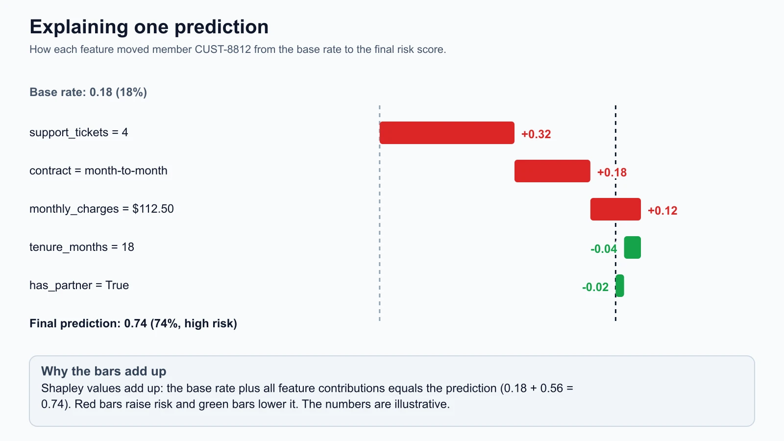
In the waterfall plot above for StayWell member CUST-8812:
- The population baseline churn rate is (18.0%).
support_tickets = 4contributes to the risk score.contract = month-to-monthcontributes .monthly_charges = $112.50contributes .tenure_months = 18offsets risk by .has_partner = Trueoffsets risk by .- The sum of all attributions () added to the baseline () equals the final prediction: (74.0%).
The boundaries of interpretability: What explanations can and cannot show
Explainability tools provide powerful operational diagnostics, but teams frequently misinterpret their statistical output, leading to severe architectural and business mistakes.
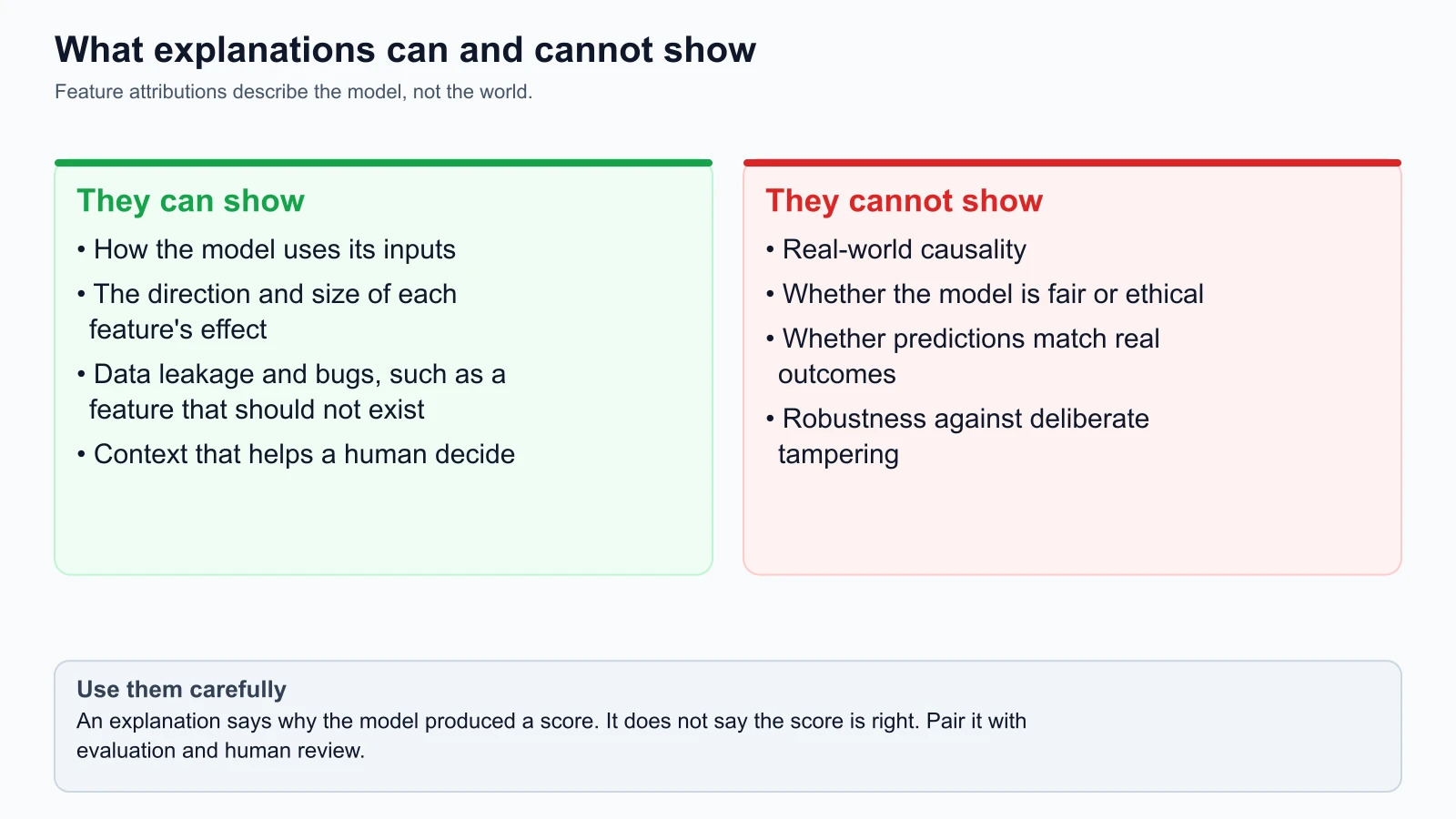
| What explanations can show | What explanations cannot show |
|---|---|
| How the model uses its inputs | Real-world causality |
| Direction and size of each feature's effect | Whether the model is fair or ethical |
| Data leakage and bugs, such as a feature that should not be available | Whether predictions are accurate against real outcomes |
| Context that helps a human operator decide | Robustness against deliberate tampering |
1. Attribution is NOT causality
This is the single most dangerous misconception in applied data science. A Shapley value reveals how much the model's mathematical function used feature to predict . It does not prove that intervening on feature will cause target to change in the physical world.
- StayWell fallacy: An engineer examines a SHAP plot showing that
monthly_chargeshas a strong positive attribution towards churn. They advise marketing to offer a 20% price cut across all at-risk customers. In reality, the high churn was driven by app crashes among premium-tier users. The price discount reduces company revenue without fixing the software bugs, and churn rates remain unchanged. - Observational model weights reflect correlations within historical training records. True causal impact requires randomized controlled trials (A/B testing) or causal inference techniques (such as instrumental variables and do-calculus).
2. Attribution does NOT prove fairness
A team might train a customer credit scoring model, omit sensitive protected attributes (such as race, religion, and gender) from the feature store, and inspect SHAP plots showing that zip_code and cell_phone_carrier drove the model decisions. The team mistakenly concludes that the model is unbiased.
In reality, non-protected features often act as high-fidelity proxies for protected demographics. SHAP attributions faithfully report that zip_code contributed to the score, but they cannot tell you whether zip_code is disproportionately penalizing historically marginalized communities. Fairness requires explicit statistical demographic audits, not feature attribution plots.
3. Explanations justify what the model believes, not what is true
If a model is trained on flawed, biased, or noisy data, its internal logic is flawed. A local explanation faithfully explains the model's corrupted reasoning. A completely incorrect model can produce elegant, convincing waterfall plots. Never confuse an explanation of a model's internal computation with real-world truth.
Fairness audits and algorithmic bias awareness
Machine learning systems in healthcare, lending, employment, and customer retention must be audited for disparate impact across demographic sub-populations.
Mature engineering teams evaluate algorithmic fairness using three standard statistical criteria:
- Demographic parity (Disparate impact): Requires that the likelihood of receiving a positive prediction (e.g. being approved for a loan or receiving a proactive customer retention discount) is equal across all demographic groups: A well-known rule of thumb is the four-fifths rule from the US federal Uniform Guidelines on Employee Selection Procedures, which says a selection rate for a group that is less than 80% of the rate for the group with the highest rate will generally be regarded as evidence of adverse impact. It was written for employment decisions, so treat it here only as a way to build a simple ratio check. It is not a legal test for a marketing offer, and this lesson is not legal advice.
- Equalized odds (Error rate parity): Requires that the model exhibit equal True Positive Rates and equal False Positive Rates across demographic groups:
- Predictive parity (Calibration): Requires that the realized probability of outcome given a predicted score is identical regardless of demographic membership.
Reviewer documentation: the model card template
Complex machine learning systems must be documented for cross-functional stakeholders, risk committees, and external compliance reviewers. In 2019, Margaret Mitchell and colleagues introduced the concept of Model Cards as standardized documentation for machine learning models.
Here is the production Model Card template used to document StayWell's customer churn model:
1# Model Card: StayWell Churn Predictor
2
3* **Model Version:** `v1.4.2`
4* **Release Date:** 2026-11-05
5* **Model Type:** LightGBM Gradient Boosted Decision Ensemble (250 trees, max depth 5)
6* **License & Access:** Internal Proprietary (StayWell Operations)
7* **Primary Owners:** Lead MLOps Engineer, Customer Data Science Team
8
9## 1. Intended Use
10* **Primary Purpose:** Identify consumer members with high risk of subscription cancellation
11  within the next 30 days.
12* **Intended Users:** Frontline customer support representatives and automated email
13  retention campaign systems.
14* **Out-of-Scope Uses:** Must NOT be used for health insurance pricing, premium
15  adjustments, or claims denial decisions.
16
17## 2. Training and Evaluation Data
18* **Training Cohort:** 450,000 anonymized member subscription records between
19  2026-01-01 and 2026-09-30.
20* **Evaluation Cohort:** 50,000 holdout member records from 2026-10-01 to 2026-10-31.
21* **Preprocessing:** Direct PII removed; numerical features median-imputed;
22  categorical variables encoded via target encodings.
23
24## 3. Quantitative Performance
25* **Validation AUC:** 0.846
26* **Brier Score (Calibration):** 0.114
27* **Precision at Top Decile:** 0.684
28* **Inference Latency (P99):** 28.4 milliseconds (4 vCPU Graviton3)
29
30## 4. Explainability and Feature Attributions
31* **Global Drivers:** `tenure_months` (28% importance), `monthly_charges` (22%),
32  `support_tickets_last_30d` (19%), `contract_type` (15%).
33* **Local Interpretability Tooling:** TreeSHAP integrated into CRM API; waterfall
34  attributions attached to all High-Risk member lookups.
35
36## 5. Fairness and Demographic Disparity Audit
37* Evaluated across user age brackets [18-30, 31-50, 51+] and geographic regions:
38  - Disparate Impact Ratio across age brackets: 0.88 (satisfies 4/5ths rule > 0.80).
39  - True Positive Rate difference between regions: < 2.5%.
40
41## 6. Caveats and Known Limitations
42* Feature attributions represent statistical correlations and must not be interpreted
43  as causal interventions.
44* Model performance degrades on newly enrolled members with tenure under 14 days due
45  to lack of historical support interaction data.
Practical code: Additive feature attribution engine
Below is a self-contained, fully tested Python implementation of a local feature attribution engine. It models linear and logistic surrogate behavior, calculates exact baseline-centered Shapley attributions, validates the game-theoretic additivity property, and formats human-readable risk explanations for frontline operations.
local_explainer.py
1"""
2Local Feature Attribution Engine.
3
4Demonstrates:
5- Baseline-centered additive feature attributions (Shapley efficiency property)
6- Directional risk attribution formatting (Increases vs Decreases Risk)
7- Absolute magnitude ranking for frontline operators
8- Pure Python standard library implementation
9"""
10
11from dataclasses import dataclass
12from typing import Dict, List, Any
13
14
15@dataclass(frozen=True)
16class FeatureAttribution:
17    """Represents a single feature attribution score."""
18    feature_name: str
19    feature_value: Any
20    attribution_value: float
21    direction: str  # "INCREASES_RISK", "DECREASES_RISK", "NEUTRAL"
22
23
24@dataclass(frozen=True)
25class LocalExplanation:
26    """Encapsulates full local explanation and verifies mathematical consistency."""
27    instance_id: str
28    base_value: float
29    prediction_value: float
30    attributions: List[FeatureAttribution]
31
32    def verify_additivity(self, tolerance: float = 1e-4) -> bool:
33        """Verify Shapley additivity: sum(attributions) == prediction - base_value."""
34        total_attribution = sum(a.attribution_value for a in self.attributions)
35        expected_delta = self.prediction_value - self.base_value
36        return abs(total_attribution - expected_delta) < tolerance
37
38
39class LinearSurrogateExplainer:
40    """
41    Computes exact additive feature attributions for linear / surrogate models.
42    Satisfies the game-theoretic efficiency and additivity axioms.
43    """
44
45    def __init__(
46        self,
47        weights: Dict[str, float],
48        intercept: float,
49        background_data: List[Dict[str, float]]
50    ):
51        self.weights = weights
52        self.intercept = intercept
53        self.background_data = background_data
54
55        if not background_data:
56            raise ValueError("Background reference dataset must be non-empty")
57
58        # Compute global expected prediction E[f(X)] over reference cohort
59        bg_scores = [self._score_raw(row) for row in background_data]
60        self.base_value = sum(bg_scores) / len(bg_scores)
61
62        # Compute baseline mean feature values E[X_i]
63        self.bg_means: Dict[str, float] = {}
64        for feature in self.weights:
65            vals = [row.get(feature, 0.0) for row in background_data]
66            self.bg_means[feature] = sum(vals) / len(vals)
67
68    def _score_raw(self, features: Dict[str, float]) -> float:
69        """Compute raw linear model score."""
70        score = self.intercept
71        for f, w in self.weights.items():
72            score += w * features.get(f, 0.0)
73        return score
74
75    def explain(
76        self,
77        instance_id: str,
78        instance_features: Dict[str, float]
79    ) -> LocalExplanation:
80        """
81        Compute additive Shapley attributions for a single instance.
82        phi_i = w_i * (x_i - E[X_i])
83        """
84        pred_value = self._score_raw(instance_features)
85        attributions: List[FeatureAttribution] = []
86
87        for f, w in self.weights.items():
88            val = instance_features.get(f, 0.0)
89            bg_mean = self.bg_means.get(f, 0.0)
90
91            # Marginal Shapley attribution for feature i in linear formulation
92            phi_i = w * (val - bg_mean)
93
94            if phi_i > 0.001:
95                direction = "INCREASES_RISK"
96            elif phi_i < -0.001:
97                direction = "DECREASES_RISK"
98            else:
99                direction = "NEUTRAL"
100
101            attributions.append(FeatureAttribution(
102                feature_name=f,
103                feature_value=val,
104                attribution_value=round(phi_i, 4),
105                direction=direction
106            ))
107
108        # Order attributions descending by absolute impact magnitude
109        attributions.sort(key=lambda a: abs(a.attribution_value), reverse=True)
110
111        return LocalExplanation(
112            instance_id=instance_id,
113            base_value=round(self.base_value, 4),
114            prediction_value=round(pred_value, 4),
115            attributions=attributions
116        )
Unit test suite verifying additivity and attribution logic
Here is the unit test suite that validates the Shapley additivity property, directionality of risk factors, and magnitude sorting:
local_explainer_test.py
1import unittest
2from local_explainer import LinearSurrogateExplainer
3
4
5class TestExplainerEngine(unittest.TestCase):
6    def setUp(self):
7        self.weights = {
8            "tenure_months": -0.04,
9            "monthly_charges": 0.02,
10            "support_tickets": 0.50,
11            "contract_two_year": -0.80
12        }
13        self.intercept = -0.20
14        # Background reference data (mean tenure: 20, mean charges: 60, mean tickets: 1)
15        self.background_data = [
16            {"tenure_months": 10, "monthly_charges": 50, "support_tickets": 0, "contract_two_year": 0.0},
17            {"tenure_months": 20, "monthly_charges": 60, "support_tickets": 1, "contract_two_year": 0.0},
18            {"tenure_months": 30, "monthly_charges": 70, "support_tickets": 2, "contract_two_year": 1.0},
19        ]
20        self.explainer = LinearSurrogateExplainer(self.weights, self.intercept, self.background_data)
21
22    def test_additivity_property_holds(self):
23        instance = {
24            "tenure_months": 5,
25            "monthly_charges": 95.0,
26            "support_tickets": 4,
27            "contract_two_year": 0.0
28        }
29        exp = self.explainer.explain("CUST-1001", instance)
30        self.assertTrue(exp.verify_additivity(tolerance=1e-3))
31
32    def test_attribution_directions(self):
33        instance = {
34            "tenure_months": 5,           # Below mean (20) -> w < 0 -> phi > 0 (Increases risk)
35            "monthly_charges": 95.0,      # Above mean (60) -> w > 0 -> phi > 0 (Increases risk)
36            "support_tickets": 4,         # Above mean (1)  -> w > 0 -> phi > 0 (Increases risk)
37            "contract_two_year": 1.0      # Above mean (0.33) -> w < 0 -> phi < 0 (Decreases risk)
38        }
39        exp = self.explainer.explain("CUST-1002", instance)
40        lookup = {a.feature_name: a for a in exp.attributions}
41
42        self.assertEqual(lookup["support_tickets"].direction, "INCREASES_RISK")
43        self.assertEqual(lookup["monthly_charges"].direction, "INCREASES_RISK")
44        self.assertEqual(lookup["contract_two_year"].direction, "DECREASES_RISK")
45
46    def test_sorting_by_magnitude(self):
47        instance = {
48            "tenure_months": 20,          # Exactly mean -> phi = 0
49            "monthly_charges": 60.0,      # Exactly mean -> phi = 0
50            "support_tickets": 5,         # Far above mean -> largest phi
51            "contract_two_year": 0.0
52        }
53        exp = self.explainer.explain("CUST-1003", instance)
54        self.assertEqual(exp.attributions[0].feature_name, "support_tickets")
55
56
57if __name__ == "__main__":
58    unittest.main()
Save both files in the same folder and run the tests from that folder:
1python3 -m unittest discover -p '*_test.py'Mistakes beginners make
1. Confusing statistical feature attribution with causal intervention
Teams routinely inspect a SHAP waterfall plot showing that high monthly_charges contributed to churn risk, and instruct marketing to give the customer a $15 discount. If the customer is actually cancelling because the mobile app crashes during workouts, lowering the price fails to stop churn while unnecessarily eroding profit margins.
Fix: Treat feature attributions as statistical evidence inside model weights, not prescriptive causal actions. Validate interventions through randomized A/B tests or formal causal inference models before implementing business policies.
2. Assuming that dropping sensitive columns eliminates demographic bias
Developers frequently remove protected attributes (such as age, gender, or race) from training datasets, assuming this guarantees fair and ethical predictions. The model easily reconstructs the omitted protected variables through correlated proxies (such as postal code, browsing device, or plan type).
Fix: Audit production predictions across demographic slices using formal fairness metrics (such as demographic parity ratios and equalized odds error checks). Removing sensitive features from training data without disparity testing creates a false sense of compliance.
3. Relying on slow KernelSHAP inside real-time inference request loops
Engineers often attempt to compute model-agnostic KernelSHAP values synchronously on every incoming online REST request. Because KernelSHAP requires generating and evaluating thousands of model permutations, inference latency spikes from 20 milliseconds to over 5,000 milliseconds, bringing down production APIs.
Fix: For tree models, use highly optimized C++ TreeSHAP implementations. For high-throughput online APIs, precalculate attributions offline during batch scoring, or compute explanations asynchronously in background workers rather than blocking real-time user HTTP responses.
4. Deploying models without standardized model cards
Data science teams often hand off trained models to production engineers via an unannotated binary file (e.g. model_final_v2.pkl) and a chat message. Months later, when risk auditors or regulators inquire about training cohorts, intended uses, or known performance limitations, nobody can locate the original records.
Fix: Mandate an approved Model Card checked into source control alongside model artifacts. Document training date ranges, quantitative performance benchmarks, intended operational scope, known edge-case failures, and demographic fairness audits.
Recap and try it yourself
In this lesson, we established the core principles of Explainable AI:
- Global versus local interpretability: Global metrics (permutation importance) audit population tendencies; local metrics (SHAP, LIME) explain individual predictions.
- Game-theoretic foundations of SHAP: Shapley values allocate prediction deltas fairly across features, uniquely guaranteeing efficiency and additivity: .
- The limits of interpretability: Explanations reveal internal model weighting, but cannot prove real-world causality, ethical fairness, or ground-truth accuracy.
- Algorithmic fairness audits: Verify disparate impact and error rate parity across demographic sub-groups.
- Model Card governance: Standardize model documentation covering intended scope, quantitative performance, fairness audits, and known operational caveats.
Hands-on exercises
- Trace an individual customer explanation:
Using the
LinearSurrogateExplainerfrom our practical code, create an explanation for a loyal subscriber:tenure_months = 48,monthly_charges = 45.0,support_tickets = 0, andcontract_two_year = 1.0. Which feature provides the strongest negative attribution (protecting against churn)? Does the additivity verification pass? - Calculate a Disparate Impact ratio: Suppose StayWell tests a proactive retention offer. Among subscribers in Group A, 120 out of 1,000 members receive the offer (12.0%). Among subscribers in Group B, 250 out of 1,000 receive the offer (25.0%). Calculate the disparate impact ratio (). Is it below the four-fifths threshold of , and what would you investigate next?
- Identify a target leakage feature via SHAP:
In a churn dataset, an engineer includes the feature
days_since_account_closed. If an active customer has never closed their account, this value is null (imputed as 999); for cancelled members, it is small. Explain what the SHAP attribution for this feature would look like, and why this represents catastrophic target leakage rather than legitimate predictive signal.