
MLOps course · lesson 1 of 24
- 1What Is MLOps? From Notebooks to Reliable Production
- 2MLOps Principles and Maturity: From Manual to Automated
- 3ML Fundamentals for MLOps: Splits, Leakage, and Metrics
- 4A Reproducible ML Project: Layout, Seeds, and Data Code
- 5Data Engineering Basics for ML: Ingestion, SQL, and Skew
- 6Pipeline Orchestration: Apache Airflow and Kubeflow
- 7Batch vs Streaming: Spark, Kafka, and Flink
- 8Data Versioning and Lineage: DVC and Beyond
- 9Data Validation and Quality in ML Pipelines
- 10Experiment Tracking with MLflow
- 11Reproducible Training Pipelines
- 12Model Evaluation and Validation Gates
- 13Model Registry and Versioning
- 14CI/CD for Machine Learning
- 15Containers and Kubernetes for ML
- 16Infrastructure as Code: Terraform and Ansible
- 17Cloud ML Platforms: AWS, Azure, GCP, and Self-Built
- 18Model Serving Patterns: Batch, Online, and Streaming
- 19Inference Engineering Basics: Latency, Batching, and Cost
- 20Monitoring and Observability for ML Models
- 21Drift Detection and Retraining for ML Models
- 22Explainable AI: LIME, SHAP, and Model Interpretability
- 23Edge AI Deployment: Jetson, TFLite, and Mobile ML
- 24Capstone: An End-to-End MLOps Pipeline
Building a machine learning model inside an interactive notebook is an engaging way to test ideas. You load a dataset, clean a few columns, train an algorithm such as a gradient boosted tree (an ensemble technique that combines multiple decision trees iteratively to correct prior errors), and observe strong validation metrics. In that isolated environment, the work looks complete.
Yet in practice, many models built in notebooks never reach production, and many that do reach production degrade silently over time. Models often struggle outside notebooks because running code in production requires far more than an optimization algorithm. A production model depends on reliable data pipelines, automated tests, version control across code and data, serving infrastructure, and ongoing monitoring.
This engineering discipline is known as Machine Learning Operations, commonly shortened to MLOps.
In this foundational lesson, you will learn what MLOps is, how it differs from traditional DevOps, why the transition from exploratory notebooks to production software fails, and how engineering discipline prevents hidden technical debt. You will also meet StayWell, the running case study and synthetic production application that anchors this entire 24-lesson course.
Defining MLOps
Machine Learning Operations (MLOps) is the engineering practice of unifying machine learning development and system operations to standardize, automate, and monitor the entire machine learning lifecycle.
MLOps applies established DevOps practices, including continuous integration, continuous delivery, automated testing, configuration management, and infrastructure as code, to the specific challenges of machine learning.
To understand why machine learning requires its own operational discipline, consider how traditional software compares to machine learning systems:
| Dimension | Traditional Software Engineering (DevOps) | Machine Learning Engineering (MLOps) |
|---|---|---|
| Primary artifacts | Code and compiled binaries | Code, data, and model parameters |
| Determinism | Deterministic: identical code with identical input yields identical output | Probabilistic: identical code on updated data yields a different model |
| Versioning target | Source code repositories (Git commits, releases) | Multi-modal: code commits, data hashes, model weights, runtime environments |
| Testing scope | Unit tests, integration tests, end-to-end user flows | Code tests, data validation contracts, evaluation gates, bias checks |
| System decay | Bugs, bit rot, dependency obsolescence | Statistical drift: data drift (covariate shift) and concept drift |
| Team profiles | Software engineers, QA testers, site reliability engineers | Data scientists, machine learning engineers, data engineers, operations teams |
Standard software behaves deterministically: if a web service handles user requests correctly on Tuesday, it will behave the same way on Wednesday as long as the code, hardware, and runtime environment remain unchanged. The business rules live directly in code written by developers.
Machine learning models derive their logic from patterns in historical training data. When customer behavior changes or external market conditions shift, the model's predictions can drift away from reality even when every line of application code remains untouched. MLOps provides the engineering practices and tooling needed to manage this continuous, data-driven cycle.
The notebook-to-production gap
Most data science initiatives begin in exploratory computing environments like Jupyter notebooks. Notebooks are helpful tools for initial hypothesis testing, exploratory data analysis, and rapid prototyping. They provide instant visual feedback, rich table displays, and inline visualizations that allow practitioners to verify quickly whether a signal exists within raw data.
However, notebooks are ill-suited for production execution. The qualities that make notebooks pleasant for ad-hoc experimentation create serious operational problems when run on production servers:
- Non-linear cell execution: Notebook cells can be executed in arbitrary order. A developer might run cell ten, backtrack to tweak cell four, run cell seven, and achieve a successful result. If the notebook is restarted from top to bottom, the code frequently breaks because variables were created out of order.
- Local path dependencies: Notebook scripts routinely rely on absolute paths pointing to local laptop directories, such as paths in local download folders. These paths do not exist inside a container running on a remote cloud cluster.
- Implicit runtime environments: Notebooks execute within a pre-existing Python kernel that accumulated libraries over months of experimentation. Without pinned dependency lockfiles, reproducing the exact runtime environment on another machine is unreliable.
- Missing test coverage: Code written in notebook cells rarely includes unit tests, input schema assertions, or boundary condition checks.
- Untracked model artifacts: Exporting a model by manually calling Python serialization and moving the resulting binary file provides zero lineage. Teams cannot trace which Git commit, which training dataset, or which hyperparameter configuration produced that specific file. A hyperparameter is a configuration setting chosen before training begins, such as the maximum depth of a decision tree or a learning rate.
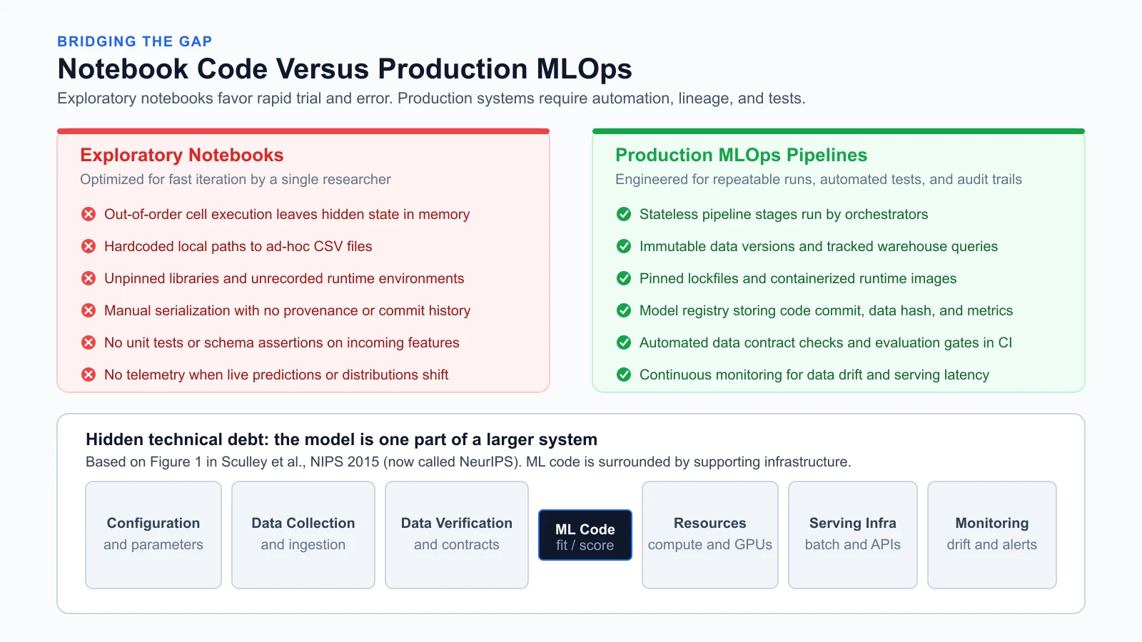
Bridging this gap means moving from manual scripting to structured pipelines. An MLOps architecture replaces manual cell execution with modular, parameterized steps; unversioned local files with immutable, hashed storage; and loose model files with a formal model registry that tracks full provenance. A model registry is a centralized store that manages model versions, metadata, and lifecycle stages.
Hidden technical debt in machine learning systems
Sculley and colleagues at Google presented their findings at NIPS 2015 (now NeurIPS) in Hidden Technical Debt in Machine Learning Systems. The paper explained that machine learning systems often carry large ongoing maintenance costs because they possess technical debt factors distinct from traditional software.
In Figure 1 of the paper, the authors illustrated that writing the mathematical model code (such as calling a fitting routine or defining neural network layers) represents only a small box at the center of the architecture. The surrounding system consists of much larger components dedicated to configuration, data collection, feature extraction, data verification, machine resource management, serving infrastructure, and monitoring.
When teams focus solely on tuning algorithms while neglecting the surrounding infrastructure, systems become fragile and expensive to maintain. The paper identifies several primary debt factors:
Entanglement and the CACE principle
In traditional modular software, encapsulation and information hiding allow developers to modify one component without breaking unrelated services. Machine learning models, by contrast, mix all input signals together during optimization. This dynamic is known as the CACE principle: Changing Anything Changes Everything.
If you add a new feature to an existing model, alter the distribution of an existing feature, or change a hyperparameter, the weights assigned to every other feature in the model can shift. You cannot tune or isolate one part of a learned model independently.
Data dependencies
In standard software, compilers and type systems enforce interfaces. In machine learning, systems consume raw data from external upstream stores. The paper identifies unstable data dependencies (where upstream data changes unexpectedly) and underutilized data dependencies (features that provide marginal benefit but high ongoing maintenance cost) as major sources of debt. When an upstream team modifies column formats or data types, the machine learning model does not throw a syntax error. Instead, it consumes the altered inputs and outputs inaccurate predictions silently.
Hidden feedback loops
Production models often influence the data collected for future training runs. For example, a recommendation system directs users toward specific items, causing future engagement data to reflect the model's own prior choices rather than unbiased user preference. Without deliberate isolation and ground-truth validation, models can reinforce their own biases over time.
Undeclared consumers
Because a model's predictions are often published to message queues or database tables, other software systems across an organization may consume those predictions without the modeling team's knowledge. If the modeling team updates the model to optimize for a new business metric, downstream systems that depended on the previous output characteristics can break unexpectedly.
Configuration debt
Machine learning pipelines involve dozens of configuration values: feature flags, learning rates, regularizers, data window boundaries, and resource limits. When configurations are scattered across command-line flags and shell scripts, verifying what settings were applied to a specific run becomes difficult.
Erosion of system boundaries
Machine learning systems frequently pull in external data sources and emit predictions across complex application workflows. When interfaces between data ingestion, model scoring, and business logic are not strictly enforced through contracts, changes in business rules bleed directly into data pipelines.
By treating data validation, configuration, orchestration, and monitoring as core engineering responsibilities, teams prevent these debt factors from accumulating.
The end-to-end machine learning lifecycle
Operating machine learning in production is an iterative lifecycle composed of distinct phases connected by automated feedback loops.
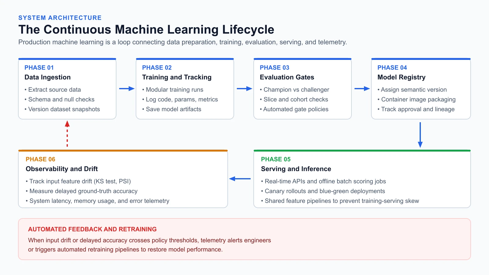
Here is how each phase functions within a complete MLOps architecture:
Phase 1: Business framing and data engineering
Every project begins by translating an operational business problem into a concrete prediction objective. Once the goal is defined, data engineering pipelines extract raw data from transactional databases, analytical warehouses, or event streams.
MLOps introduces automated data validation at this entry point. Incoming data is verified against a data contract, which is a formal agreement specifying expected schemas, null tolerances, value ranges, and update frequencies. Datasets are versioned using cryptographic hashes so that any training run can be reconstructed precisely.
Phase 2: Model training and experiment tracking
With validated data available, modeling begins. Training code is structured into modular pipeline stages managed as a Directed Acyclic Graph (DAG), a set of tasks with dependencies between them and no loops, so each task runs only after the tasks it depends on have finished.
Data scientists explore multiple configurations: adjusting feature transformations, testing algorithms, and tuning hyperparameters. MLOps experiment tracking systems record every run automatically, logging the exact Git commit, input data hash, hyperparameters, training duration, and evaluation metrics. Every candidate model artifact is stored alongside its complete execution context.
Phase 3: Evaluation and validation gates
Before any model serves production traffic, it must pass through automated evaluation gates. Achieving a higher average score on a test set is not sufficient.
MLOps validation suites perform slice-based evaluation, verifying that a candidate model does not perform unacceptably poorly on high-value customer tiers or rare edge cases. Candidate models (challengers) are evaluated directly against the currently deployed model (champion). Evaluation gates verify multiple metrics:
- Precision: the proportion of positive predictions that were correct.
- Recall: the proportion of actual positive cases that were correctly identified.
- Area Under the ROC Curve (AUC): a metric measuring how well a classifier separates positive and negative classes across all classification thresholds.
- F1-Score: the harmonic mean of precision and recall, balancing false alarms against missed events.
If a candidate model fails any threshold, the release pipeline stops automatically.
Phase 4: Model registry and packaging
Models that pass validation gates are registered into a centralized model registry. The registry acts as an immutable catalogue of record. It assigns semantic version numbers, tracks approvals, and records deployment readiness stages such as Staging or Production.
The model artifact is packaged alongside its runtime dependencies into a standardized container image. This guarantees that the scoring logic behaves identically across development, testing, and production clusters.
Phase 5: Inference and serving patterns
Once registered, the model is deployed to inference infrastructure. Depending on the operational requirement, serving follows one of three patterns:
- Batch inference: scheduled jobs that score large sets of records offline and write predictions to an analytical table or cache.
- Real-time API inference: low-latency web services (using REST or gRPC, a high-performance remote procedure call framework communicating over HTTP/2) that score individual requests in milliseconds.
- Streaming inference: event-driven consumers that process messages from distributed message logs in near real time.
Production deployments use gradual rollout strategies to limit operational risk. In a canary release, a new model receives a small percentage of live traffic before rolling out broadly. In a blue-green deployment, two identical environments run side by side, allowing instant switching between versions.
Serving pipelines also guard against training-serving skew, which is a discrepancy between how features are calculated during offline training and how they are calculated in live production inference. Teams often use a feature store (a centralized platform that calculates and serves curated features) to keep training and serving data consistent.
Phase 6: Observability, drift detection, and retraining
Deployment begins the operational monitoring phase. Telemetry infrastructure monitors system health (latency, memory usage, CPU/GPU utilization, and error rates) and data integrity.
Because ground-truth labels often arrive with substantial delays, MLOps systems monitor input distributions directly. Two primary forms of drift occur in production:
- Data drift (covariate shift): the distribution of input features changes over time while the underlying relationship between inputs and outputs remains the same.
- Concept drift: the actual statistical relationship between input features and target labels changes over time.
Teams detect drift using statistical techniques such as the Kolmogorov-Smirnov test (KS test, a non-parametric test comparing the cumulative distributions of two continuous datasets) and the Population Stability Index (PSI, a metric that quantifies how much a variable's distribution has shifted away from a reference baseline).
When drift metrics cross predefined thresholds, automated alerts notify engineers, or automated continuous retraining pipelines trigger to update the model on fresh data.
Team roles and collaboration
A frequent cause of friction in machine learning initiatives is ambiguity regarding team ownership. Handing unverified prototype code from data science to software developers to re-implement from scratch is inefficient and introduces subtle bugs.
A structured MLOps practice establishes clear ownership across four complementary roles:
| Role | Primary ownership | Typical deliverables |
|---|---|---|
| Data Engineer | Upstream ingestion, storage, and feature pipelines | Validated feature tables, warehouse queries, streaming pipelines |
| Data Scientist | Business hypothesis, feature engineering, and algorithm exploration | Training code, experiment logs, candidate model artifacts |
| Machine Learning Engineer | Packaging, pipeline orchestration, serving infrastructure, and CI/CD | Automated training DAGs, inference APIs, validation gates, drift detectors |
| Platform / DevOps Engineer | Infrastructure provisioning, cluster management, and system monitoring | Kubernetes clusters, cloud permissions, container registries, Prometheus alerts |
In smaller teams, an individual engineer may take on multiple responsibilities. Regardless of team size, defining where data preparation ends, where modeling begins, and where deployment operations take over prevents confusion and deployment delays.
Common misunderstandings about MLOps
Teams new to MLOps often misjudge what the discipline requires:
- Packaging code in a container is only one step: Putting an unversioned script into a Docker container solves runtime dependencies, but it does not address data validation, experiment lineage, evaluation gates, drift detection, or retraining workflows.
- Buying software platforms does not replace engineering discipline: Purchasing an enterprise tool does not compensate for missing unit tests, undefined data contracts, or vague deployment criteria.
- MLOps differs fundamentally from standard DevOps: Traditional DevOps assumes deterministic code execution and static test suites. Machine learning systems decay due to environmental data shifts even when application code remains untouched.
- MLOps applies to teams of all sizes: You do not need large distributed clusters to benefit from basic operational habits like pinning dependencies, fixing random seeds, writing schema assertions, and recording model versions.
Meet StayWell: a running production case study
Throughout this course, every architectural pattern, code template, and deployment workflow will be applied to a single production case study: StayWell.
StayWell is fictional; all data in this course is synthetic and generated by our own code.
The business scenario
StayWell operates a subscription fitness and wellness mobile application. Customers pay a monthly membership fee to access personalized workout plans, wellness tracking, and a direct coaching chat.
The operational problem facing StayWell is customer churn: members cancelling their monthly memberships. Acquiring new subscribers requires marketing expenditure, so retaining existing members keeps revenue stable.
StayWell's member success team wants to intervene proactively. If an automated machine learning system can identify which subscribers are at high risk of cancelling within the next thirty days, the team can offer targeted interventions, such as a personalized workout plan adjustment or an engagement check-in.
Operational constraints and requirements
Operating StayWell's churn prediction model introduces realistic engineering constraints:
- Input features: Subscriber account data (membership tier, age, signup tenure), behavioral usage metrics (weekly workouts logged, coach messages sent, app login frequency), and billing history (past discount codes applied, failed payment attempts).
- Dual serving architecture: The system requires both batch scoring (scoring all active members every Sunday evening to populate the member success dashboard) and real-time scoring (evaluating churn risk immediately when a user navigates to the membership cancellation settings page).
- Latency budget: Real-time scoring requests must return predictions in under one hundred milliseconds.
- Balanced evaluation metrics: A false positive flags a customer who would have stayed, spending retention budget unnecessarily on unneeded discounts. A false negative misses a customer who actually cancels, resulting in lost subscriber revenue. The evaluation gate must balance precision and recall across subscriber tenure tiers.
- Seasonal drift: In our fictional scenario, subscriber workout habits follow seasonal shifts, such as a January surge in workout motivation followed by drop-offs in February. The system must detect these input distribution shifts before prediction quality degrades.
In the lesson on the reproducible ML project, you will write the StayWell data generator. The script will produce statistically consistent, fully reproducible customer records using fixed random seeds. Because all data is generated locally by code, there are no proprietary datasets to download and no external credentials required.
Over the coming lessons, we will build a complete MLOps toolkit in Python: validating StayWell's incoming data, tracking experiments, enforcing validation gates, registering versioned models, serving predictions, and monitoring for drift.
Sources
Checked on 4 November 2026:
- D. Sculley, G. Holt, D. Golovin, E. Davydov, T. Phillips, D. Ebner, V. Chaudhary, M. Young, J.-F. Crespo, and D. Dennison, Hidden Technical Debt in Machine Learning Systems, Advances in Neural Information Processing Systems 28 (NIPS 2015).
Mistakes beginners make
When engineering teams first implement MLOps workflows, they frequently encounter several common pitfalls:
1. Adopting complex distributed tools prematurely
Teams often spend months installing complex distributed orchestration platforms before shipping their first model to production. The maintenance overhead of managing cluster infrastructure drains time from core modeling goals.
Fix: Start simple. Begin with clean Python project structures, Git versioning, lightweight experiment tracking, and automated unit tests. Introduce distributed platforms only when data scale demands it.
2. Allowing training-serving skew to enter feature calculations
A data scientist might calculate rolling averages in a notebook using vectorized batch operations, while backend engineers re-implement the same logic in an API service using different floating-point handling or timestamp boundaries. The resulting feature differences degrade model accuracy.
Fix: Implement feature calculations in shared, versioned libraries or feature pipelines that are tested and used identically in both training and serving environments.
3. Relying entirely on global accuracy
A churn prediction model that achieves ninety-five percent accuracy on an imbalanced dataset where only five percent of users churn is no better than a trivial script that predicts no one will ever churn.
Fix: Evaluate models using domain-appropriate metrics such as Precision, Recall, AUC, and F1-Score, and always measure performance across individual customer slices.
4. Failing to detect silent degradation
When standard software services fail, they return error codes or crash. When a machine learning model encounters drifted data, it returns successful HTTP 200 responses containing confident but inaccurate predictions.
Fix: Deploy telemetry that monitors the statistical distributions of incoming features and prediction scores, treating distribution shifts as operational anomalies.
Recap and try it yourself
In this foundational lesson, you explored the core tenets of MLOps:
- MLOps is the engineering discipline that bridges data science experimentation and dependable production software.
- The notebook-to-production gap arises from hidden state, unpinned environments, and missing automated tests.
- Machine learning code is a small component within a larger system of data verification, pipeline orchestration, and monitoring infrastructure.
- The machine learning lifecycle is a continuous loop connecting data ingestion, training, evaluation gates, registries, serving, and telemetry.
- StayWell provides a concrete, fictional fitness subscription case study for predicting customer churn across batch and real-time inference patterns.
Try it yourself
To apply these concepts, work through these exercises:
- Audit a script: Review a machine learning script or notebook you have previously written. How many hardcoded file paths or unpinned library versions are present? List three concrete steps you would take to make that script fully reproducible on a clean machine.
- Analyze the CACE principle: In the StayWell churn scenario, suppose you add a new feature:
coach_messages_sent_last_30_days. If the product team updates the mobile app to include automated welcome messages in that counter, explain how this change could alter the weights of other features during the next training run. - Contrast failure modes: Compare how a traditional database connection timeout appears in application logs versus how an unannounced change in incoming feature scale (such as tenure logged in days instead of months) appears in an inference service.
Next, you will look at the principles and maturity levels that let you judge any ML system.