Data Engineering Basics for ML: Ingestion, SQL, and Skew

In our previous lessons on reproducible project layout and synthetic data generation, we created clean, local data generation scripts. In production organizations, however, data scientists and machine learning engineers rarely work from a static local file. Machine learning models feed on data that originates in operational databases, distributed event logs, and external webhooks.

Before a feature reaches a scikit-learn pipeline or deep learning model, it travels through an extensive data engineering infrastructure. If that infrastructure calculates rolling averages improperly, leaks future timestamps, or shifts data types, the model fails regardless of the algorithm chosen.

In this lesson, you will learn the data engineering fundamentals that underpin machine learning: how data is ingested, how ETL differs from modern ELT, how data lakes and analytical warehouses store records, how to author point-in-time SQL feature pipelines, and how to eliminate training-serving skew. We will examine how raw application events from StayWell, our running subscription case study, are transformed into clean features for churn prediction.

Upstream data sources and ingestion patterns

Machine learning features originate across distinct operational layers:

• Transactional databases: Application backends write user profiles, account statuses, and settings to relational stores such as PostgreSQL or MySQL. These systems prioritize high-throughput atomic transactions, not complex analytical aggregations across millions of rows.
• Event logs and message streams: User activity, such as completing a workout, opening a mobile screen, or sending a coach message, generates event streams published to distributed logs like Apache Kafka or AWS Kinesis.
• Third-party webhooks: Systems like payment gateways (Stripe) emit webhooks for subscription renewals, credit card failures, and chargebacks.

Ingestion is the automated process of capturing and moving raw data from these operational systems into centralized storage without impacting user-facing production databases.

Ingestion occurs through two main patterns:

1. Batch ingestion: Periodic queries (such as nightly database snapshots or scheduled log dumps) extract changes and append them to analytical storage. Batch ingestion is straightforward and cost-effective for features that change slowly, like monthly account status.
2. Streaming ingestion: Continuous real-time consumers read messages off an event log as they happen and write them directly to storage within seconds. Streaming ingestion is required for low-latency features, like detecting immediate fraud attempts or tracking live workout progress.

ETL versus ELT: how data pipelines evolved

Historically, data integration followed the ETL (Extract, Transform, Load) pattern. Engineers extracted data from source databases, transformed it on an external compute server (such as an Apache Spark cluster or custom Python scripts), and loaded the cleaned, pre-calculated tables into a relational destination.

ETL carried significant trade-offs: the external transformation server was complex to scale, and if downstream modeling teams discovered they needed a raw field that was discarded during transformation, the entire pipeline had to be re-engineered from scratch.

Modern data platforms have largely transitioned to ELT (Extract, Load, Transform):

1ETL:  [Source DB]  -->  [External Transform Server]  -->  [Clean Warehouse Table]
2                                (Data Discarded)
3
4ELT:  [Source DB]  -->  [Raw Data Lake / Warehouse]  -->  [SQL Transformation Engine]
5                                (Raw Data Preserved)

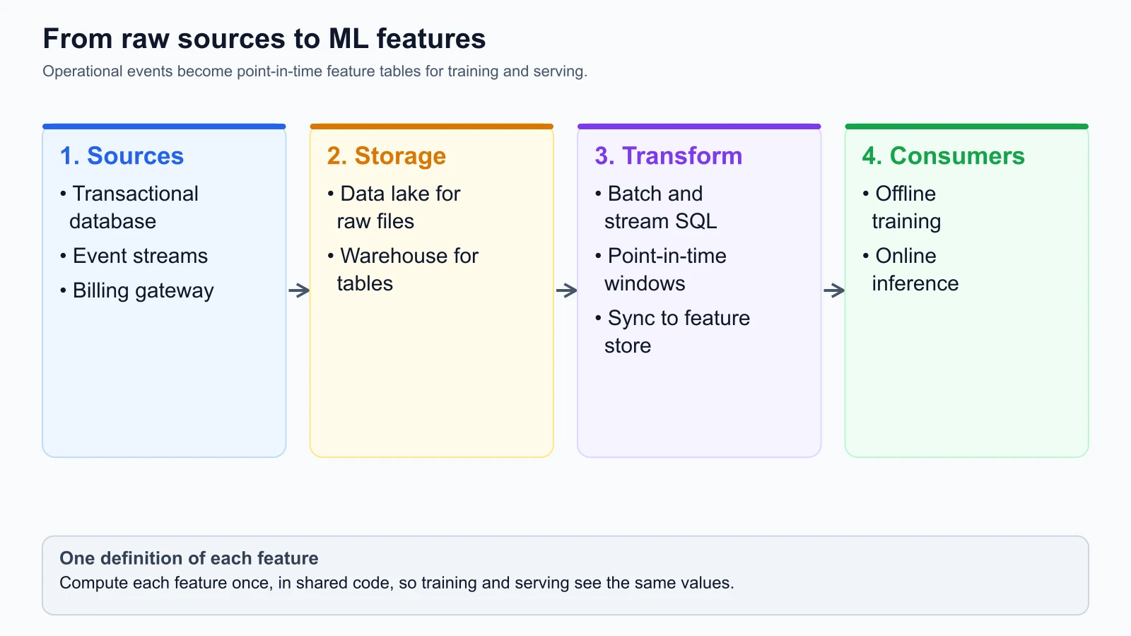
In ELT, ingestion tools extract data and load it in its raw format directly into storage. Transformations execute downstream inside modern analytical warehouses using SQL or tools like dbt (data build tool).

ELT provides three operational advantages for machine learning:

• Raw history preservation: Because raw events remain stored in the lake, data scientists can engineer novel features from historical events without asking data engineers to modify upstream ingestion.
• Elastic compute scale: Analytical warehouses like Snowflake, BigQuery, and Databricks scale compute resources independently, executing aggregations over billions of rows in minutes.
• Auditable lineage: Transformations are written in version-controlled SQL, allowing teams to audit exactly how every feature was derived.

Data lakes, warehouses, and the lakehouse architecture

Where should ingested data live? Modern data platforms utilize three storage patterns:

Data lake

A data lake is a centralized repository that stores raw, semi-structured, and unstructured data (such as JSON payloads, CSV logs, audio, and images) in object storage like Amazon S3 or Google Cloud Storage. Data lakes offer low-cost, virtually unlimited storage, but they lack native indexing, ACID transaction guarantees, and fast SQL query performance.

Data warehouse

A data warehouse is an analytical database optimized for reading and aggregating structured tabular data using columnar storage. Examples include Snowflake, Google BigQuery, and ClickHouse. Data warehouses provide fast SQL performance, strict schema enforcement, and role-based access control, but storing raw multi-terabyte log dumps can be expensive.

Lakehouse

To bridge this divide, many modern platforms adopt a lakehouse architecture. A lakehouse combines the low-cost, scalable object storage of a data lake with open table formats (such as Delta Lake, Apache Iceberg, or Apache Hudi) that provide ACID transactions, schema enforcement, and time-travel querying.

In an MLOps pipeline, raw event streams land in the lakehouse storage tier, where automated SQL pipelines transform them into structured feature tables.

Schema evolution and data contracts

Data schemas do not remain static. Application development teams regularly update backend databases: renaming columns, modifying enum types, or adding nullable fields.

In traditional software, changing a database schema triggers migration scripts. In machine learning, however, downstream feature pipelines often consume tables across departments without direct notification.

If an engineering team alters a column from tenure_days to tenure_months or changes an enum value from "basic" to "tier_1", the machine learning pipeline does not throw an upfront syntax error. Instead, feature scalers and decision trees receive unexpected zeros or unknown category tokens, causing prediction accuracy to drop silently.

To prevent this failure mode, teams implement data contracts. A data contract is a formal specification agreed upon between the data producer (the application team) and the data consumer (the machine learning team) defining:

• Column names and strict data types.
• Allowed categorical values and null thresholds.
• Update frequency and expected row arrival latency.
• Versioning policies when schema changes are introduced.

Automated pipelines run schema assertions against these contracts before executing training or feature generation jobs.

SQL for machine learning feature engineering

While data scientists frequently prototype feature calculations using pandas, in-memory Python processing struggles when datasets exceed available RAM. In production, feature engineering over large historical event datasets is best performed inside the analytical warehouse using SQL.

Point-in-time correctness

The single most important principle in ML feature engineering is point-in-time correctness. Point-in-time correctness means that any feature calculated for a historical sample must use only the data that was known at the exact cutoff timestamp of that event.

If you calculate a subscriber's average workout count by averaging all workouts up to today, you leak future workout activity into the historical training sample. The model learns to predict based on future behavior that cannot exist when evaluating a live subscriber.

Worked example: StayWell feature generation in SQL

Let us see how raw activity events from StayWell are transformed into clean, point-in-time features using SQL window functions.

StayWell maintains two source tables in its analytical warehouse:

1. dim_subscribers: Subscriber IDs, signup dates, and membership tiers.
2. fact_workout_logs: Individual logged workout records with timestamps.

Here is the production SQL query calculating 30-day activity features without leakage:

1WITH prediction_cutoffs AS (
2    -- Establish observation cutoff dates for each subscriber
3    SELECT
4        user_id,
5        signup_date,
6        membership_tier,
7        observation_date
8    FROM dim_subscribers
9),
10
11activity_window AS (
12    -- Join workouts occurring strictly within the 30-day window before cutoff
13    SELECT
14        c.user_id,
15        c.observation_date,
16        c.membership_tier,
17        DATEDIFF('month', c.signup_date, c.observation_date) AS tenure_months,
18        COUNT(w.workout_id) AS workouts_completed_last_30d,
19        COALESCE(SUM(w.duration_minutes), 0) AS total_workout_minutes_30d,
20        MAX(w.completed_at) AS last_workout_timestamp
21    FROM prediction_cutoffs c
22    LEFT JOIN fact_workout_logs w
23        ON c.user_id = w.user_id
24        -- Strict point-in-time boundary: between 30 days prior and cutoff
25        AND w.completed_at >= DATEADD('day', -30, c.observation_date)
26        AND w.completed_at < c.observation_date
27    GROUP BY
28        c.user_id,
29        c.observation_date,
30        c.membership_tier,
31        c.signup_date
32)
33
34SELECT
35    user_id,
36    membership_tier,
37    tenure_months,
38    workouts_completed_last_30d,
39    total_workout_minutes_30d,
40    -- Calculate days since last active workout up to the observation cutoff
41    COALESCE(DATEDIFF('day', last_workout_timestamp, observation_date), 999) AS days_since_last_workout
42FROM activity_window;

This SQL query guarantees point-in-time isolation. Because w.completed_at < c.observation_date enforces an upper temporal boundary, workout events that occurred after the cutoff timestamp cannot leak into the features.

Feature tables and feature stores

As organizations deploy multiple machine learning models, individual teams often write duplicate SQL scripts to calculate the same core entities: user tenure, 30-day activity, and billing history.

To eliminate redundant computation and standardize definitions, teams organize features into feature tables. A feature table is a versioned, curated table where rows represent distinct entities (such as a subscriber or transaction) and columns represent engineered mathematical features.

When systems must serve predictions both in offline batches and in low-latency online APIs, teams adopt a feature store (such as Feast, Hopsworks, or managed cloud feature stores).

A feature store maintains two synchronized storage tiers:

• Offline store: High-capacity columnar storage (Parquet files in S3 or warehouse tables in BigQuery/Snowflake). Used by model training pipelines to extract point-in-time training datasets over years of historical data.
• Online store: Low-latency key-value storage (Redis, DynamoDB, or Cassandra). Used by live inference endpoints to look up current feature vectors for a subscriber in under ten milliseconds using their user_id.

A feature store guarantees that the exact same feature transformation logic populates both the offline and online stores, preventing mathematical discrepancies.

Training-serving skew: causes and architectural solutions

Training-serving skew is a discrepancy between the performance of a model during offline development and its performance in live production serving. It is one of the most insidious failure modes in machine learning because the service continues running without reporting errors, yet generates flawed predictions.

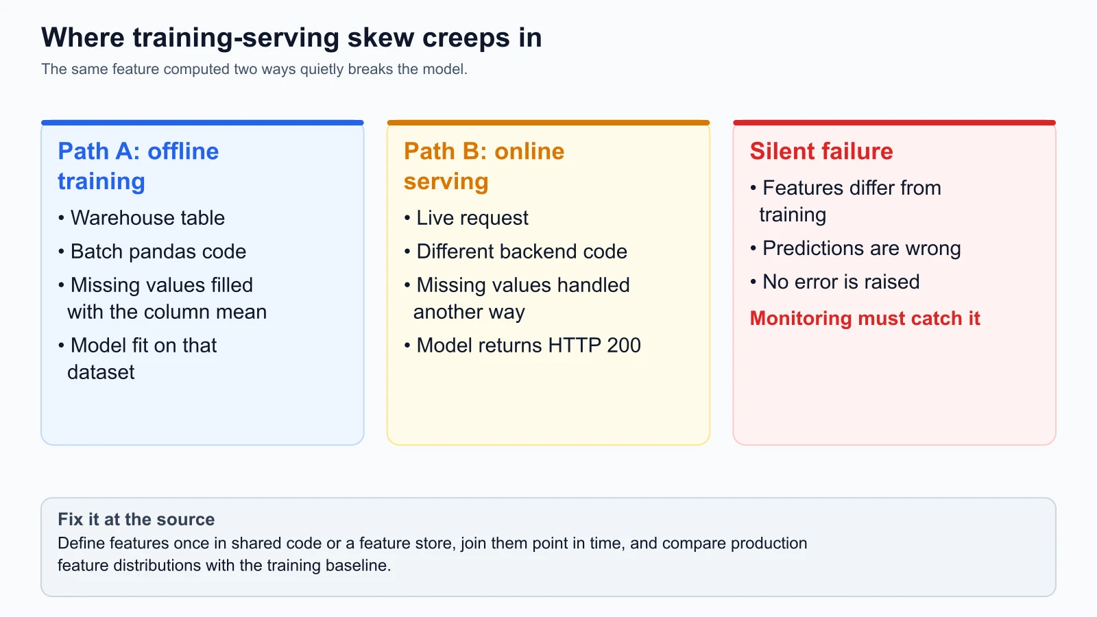
As illustrated in the diagram above, skew typically arises across three primary fault lines:

1. Implementation skew (code divergence)

A data scientist writes feature logic in Python using pandas methods for training:

1# Training code (Python/pandas)
2df["avg_workouts"] = df["workouts"].rolling(30).mean().fillna(0)

Meanwhile, backend software engineers re-implement that calculation in Go or Java inside the live API microservice:

1// Production serving code (Go)
2var avgWorkouts float64 = float64(totalWorkouts) / 30.0

Subtle differences in how missing values are handled, how time boundaries are rounded, or how floating-point division is cast create discrepancies. The model receives feature numbers that deviate from what it learned during training.

2. Time skew and point-in-time leakage

Training pipelines aggregate historical data across wide calendar windows. If the training query inadvertently includes records logged after the prediction event, the model learns to rely on future indicators that are absent during live inference.

When a live request arrives, the production endpoint can only inspect data available up to that exact millisecond. The model fails because the real-world features lack the future signals it expected.

3. Data source and distribution skew

Training datasets are often constructed from analytical warehouse tables that undergo nightly batch deduplication, validation, and reconciliation. In contrast, online serving APIs inspect raw, unvalidated telemetry directly from live event buses or user device payloads. Differences in data cleanliness, timezone handling, or null defaults degrade model predictions.

Architectural solutions to eliminate skew

To prevent training-serving skew, mature MLOps teams apply three technical safeguards:

1. Single feature definition: Write feature transformations once in a shared library or declarative feature store definition. That single code definition compiles to both batch queries for training and streaming pipelines for online serving.
2. Point-in-time joins (time-travel): Enforce strict temporal cutoffs in feature queries so training features mirror the exact data availability of production inference requests.
3. Parity telemetry: Log the exact feature vector received by production endpoints during live scoring. Asynchronously compare the distribution of live features against the baseline training distribution to detect discrepancies immediately.

Sources

Checked on 4 November 2026:

• Google for Developers, Rules of Machine Learning, which discusses training-serving skew and reusing code between training and serving.
• Feast Feature Store Documentation, Concepts overview, including offline and online stores.
• Snowflake Documentation, Window Functions Syntax and Usage.

Mistakes beginners make

When designing data pipelines and features for machine learning, engineering teams commonly make several errors:

1. Performing feature engineering after the train-test split in ad-hoc notebooks

Data scientists often write complex pandas transformation functions inside individual notebook cells that are never shared with production systems. When the time comes to deploy, backend developers must reverse-engineer the logic from scratch, introducing implementation bugs.

Fix: Write feature transformations in modular, version-controlled SQL queries or shared Python packages. Use pipeline orchestrators to generate feature tables before training.

2. Overlooking point-in-time constraints in training SQL

Engineers frequently join historical labels with customer activity using a simple JOIN on user_id without filtering on event timestamps. This leaks activity from after the churn event into the training features, creating inflated validation scores that collapse in production.

Fix: Always include strict timestamp cutoffs in feature queries (event_timestamp < prediction_cutoff_date) to ensure historical features reflect only what was observable at the decision moment.

3. Using raw operational databases for model training

Running heavy analytical aggregation queries directly against production PostgreSQL or MySQL transactional databases strains database CPU and memory, risking application downtime for end users.

Fix: Ingest transactional data into an analytical warehouse or data lake using read replicas or change data capture (CDC), and execute compute-heavy feature queries on isolated analytical storage.

4. Failing to monitor feature parity between offline and online stores

Teams often assume that features served from Redis in real time match features extracted from Snowflake for training. When subtle timestamp parsing differences occur, models silently degrade.

Fix: Sample and log live inference feature payloads to a monitoring sink. Periodically run automated drift tests comparing live feature distributions against historical training distributions.

Recap and try it yourself

In this lesson, you covered the data engineering foundations required for machine learning:

• Data moves from transactional databases, event streams, and webhooks into centralized storage through batch or streaming ingestion.
• Modern ELT architecture preserves raw data in data lakes and analytical warehouses, executing feature transformations in scalable SQL engines.
• Schema evolution must be managed using formal data contracts to prevent silent downstream pipeline failures.
• SQL window functions enable point-in-time feature engineering, preventing future data from contaminating historical training sets.
• Feature stores maintain synchronized offline and online storage tiers to prevent training-serving skew.

Try it yourself

To apply these data engineering concepts to StayWell, work through these exercises:

1. Spot the point-in-time violation: In the StayWell feature generation SQL query above, suppose an engineer changes the window filter to w.completed_at <= CURRENT_DATE(). What happens when this query is run on historical subscriber cohorts from six months ago?
2. Design an ELT feature table: For StayWell's coaching chat feature, write a conceptual SQL aggregation query that counts how many coach messages a subscriber sent in the last 7 days versus the previous 14 to 30 days. How does the ratio between these two numbers capture declining engagement?
3. Audit for implementation skew: Imagine your training pipeline computes app_logins_per_week using integer division (logins // 4), while your production API calculates it using floating-point division (logins / 4.0). For a subscriber with 10 monthly logins, how does this discrepancy affect model predictions?

In the next lesson, we will explore pipeline orchestration with Apache Airflow and Kubeflow, learning how to schedule, retry, and manage multi-step DAG workflows reliably.