
MLOps course · lesson 21 of 24
- 1What Is MLOps? From Notebooks to Reliable Production
- 2MLOps Principles and Maturity: From Manual to Automated
- 3ML Fundamentals for MLOps: Splits, Leakage, and Metrics
- 4A Reproducible ML Project: Layout, Seeds, and Data Code
- 5Data Engineering Basics for ML: Ingestion, SQL, and Skew
- 6Pipeline Orchestration: Apache Airflow and Kubeflow
- 7Batch vs Streaming: Spark, Kafka, and Flink
- 8Data Versioning and Lineage: DVC and Beyond
- 9Data Validation and Quality in ML Pipelines
- 10Experiment Tracking with MLflow
- 11Reproducible Training Pipelines
- 12Model Evaluation and Validation Gates
- 13Model Registry and Versioning
- 14CI/CD for Machine Learning
- 15Containers and Kubernetes for ML
- 16Infrastructure as Code: Terraform and Ansible
- 17Cloud ML Platforms: AWS, Azure, GCP, and Self-Built
- 18Model Serving Patterns: Batch, Online, and Streaming
- 19Inference Engineering Basics: Latency, Batching, and Cost
- 20Monitoring and Observability for ML Models
- 21Drift Detection and Retraining for ML Models
- 22Explainable AI: LIME, SHAP, and Model Interpretability
- 23Edge AI Deployment: Jetson, TFLite, and Mobile ML
- 24Capstone: An End-to-End MLOps Pipeline
Software code does not rust. A compiled Go binary or a Python microservice that executes correctly today will execute identically ten years from now as long as its operating system and hardware remain intact.
Machine learning systems are fundamentally different. A model embodies a frozen statistical snapshot of real-world relationships captured at the moment its training dataset was collected. Because human behavior, macroeconomic conditions, market competition, and seasonal trends evolve constantly, all production machine learning models degrade over time.
When StayWell launched their churn prediction model, its Area Under the ROC Curve (AUC) stood at an impressive 0.846 on validation datasets. Six months later, the marketing team noticed that retention campaigns were failing to curb cancellations. When data scientists audited the production logs, they discovered realized AUC had silently collapsed to 0.682. The engineering team panicked: they immediately triggered an automated retraining script on the preceding two weeks of raw data, deployed the newly fitted model directly to production without validation gates, and caused an even steeper drop in retention accuracy.
In this lesson, we master statistical drift detection and establish disciplined automated retraining workflows. We analyze the mathematical distinctions between data drift, concept drift, and label shift. We implement the Population Stability Index (PSI) and two-sample statistical tests. We design safe retraining pipelines with automated promotion gates, explore data windowing strategies, and establish a production Retraining Runbook that replaces operational panic with reproducible verification.
The StayWell figures in this lesson (rates, scores, counts and prices) are made up for illustration. They show how to read the numbers, not what real systems achieve.
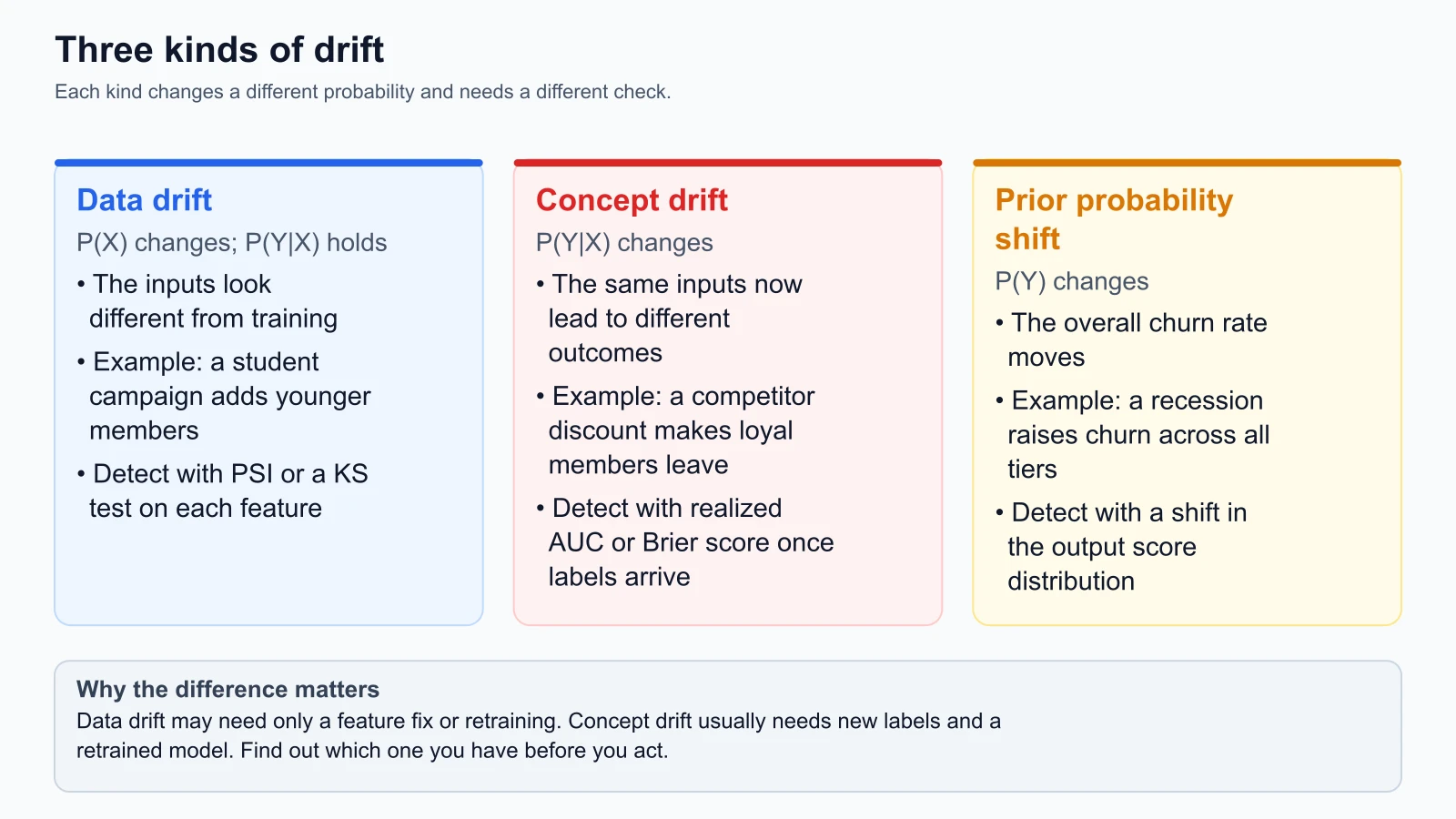
The anatomy of drift: Three distinct statistical failure modes
When a production model begins delivering inaccurate predictions, engineers often refer vaguely to "model drift." In statistical learning theory, performance degradation stems from three mathematically distinct mechanisms:
| Drift type | What shifts | Does P(Y|X) still hold? | Typical root cause |
|---|---|---|---|
| Data drift (covariate shift) | P(X), the input distribution | Yes | The mix of users changes |
| Concept drift | P(Y|X), the relationship between inputs and the label | No | Market or behavior changes |
| Prior probability shift (label drift) | P(Y), the overall target rate | Often | Macro shocks and seasons |
1. Data drift (Covariate shift)
Data drift occurs when the probability distribution of incoming input features changes over time, while the conditional probability distribution mapping features to target outcomes remains constant:
- StayWell scenario: StayWell executes a nationwide marketing campaign targeting university students. As thousands of younger users enroll, the median customer tenure drops from 24 months down to 4 months, and average monthly charges drop from $65 to $25. The input distribution has shifted dramatically. However, a 4-month subscriber paying $25 still exhibits the exact same conditional probability of churning as a 4-month subscriber did six months ago.
- Remediation: The model does not necessarily need architectural redesign; it needs to be retrained on an updated feature distribution that reflects the newly expanded customer demographic.
2. Concept drift (Relationship mutation)
Concept drift occurs when the fundamental relationship between input features and the target label changes over time, regardless of whether the input distribution shifted:
- StayWell scenario: A major competitor enters StayWell's market offering a 50% lifetime discount with zero cancellation fees. Historically, a customer with a two-year contract and high monthly usage had a negligible 4% probability of churning. Following the competitor's launch, that exact same customer profile now exhibits a 42% probability of churning. The mathematical relationship the model learned during training is no longer true in the real world.
- Remediation: Concept drift requires urgent model retraining. In severe cases, it demands engineering new features (such as competitor price ratio or recent plan comparison page views) because existing features no longer provide sufficient predictive signal.
3. Prior probability shift (Label drift)
Prior probability shift occurs when the overall base rate of the target label changes across the entire population:
- StayWell scenario: A sudden macroeconomic recession forces households to cut discretionary subscription expenditures. Overall churn jumps from 15% across the entire member base to 35%, regardless of tenure or plan type.
- Remediation: The model's raw probability predictions will be miscalibrated (under-predicting risk), requiring Bayesian prior adjustments or probability recalibration via Platt scaling or isotonic regression.
Statistical detection methods: population stability index and two-sample tests
To detect drift before real-world business losses accumulate, teams monitor feature distributions using formal statistical metrics.
Population stability index (PSI) deep dive
The Population Stability Index (PSI) is the industry standard metric for measuring divergence between a reference distribution (e.g. baseline training data) and a target distribution (e.g. current production data).
To calculate PSI:
- Divide the reference dataset into quantiles (typically 10 deciles, each containing exactly 10% of training records).
- Use those exact bin boundaries to bin the target production dataset.
- Calculate the proportion of records falling into each bin for the reference dataset (, Expected) and the target dataset (, Actual).
- Apply the PSI summation across all bins:
Notice the mathematical properties of the formula:
- If a bin has identical proportions in both datasets (), then , and the bin contributes exactly to the total index.
- If , both and are positive, yielding a positive contribution.
- If , both and are negative, and their product is also positive.
- Therefore, every discrepancy increases the total PSI value.
| PSI value | Common interpretation | Suggested action |
|---|---|---|
| Below 0.10 | No significant shift | Baseline is stable; no action |
| 0.10 up to 0.20 | Moderate shift | Log a warning and triage |
| 0.20 or higher | Significant shift | Trigger a retraining alert and investigate the root cause |
The 0.10 and 0.20 cut-offs are a widely used rule of thumb, not a law. Tune them to your data and your tolerance for false alarms.
Two-sample hypothesis tests
In addition to PSI, teams employ formal non-parametric hypothesis tests:
- Kolmogorov-Smirnov (KS) test (Continuous features): Compares the empirical cumulative distribution functions (eCDFs) of reference and target samples. The test statistic represents the maximum vertical distance between the two cumulative curves. If the p-value falls below an alpha threshold (e.g. ), the null hypothesis that both samples originate from the same continuous distribution is rejected.
- Chi-Square goodness-of-fit test (Categorical features): Compares observed categorical frequency counts against expected frequencies derived from the baseline distribution.
The sample size trap: Mitigating false alarms
A critical operational challenge with statistical hypothesis tests (such as KS and Chi-Square) is sample size sensitivity.
In production systems handling millions of requests, hypothesis tests possess extreme statistical power. A microscopic, clinically meaningless shift in average tenure (e.g. shifting from 24.00 months to 24.05 months across records) will yield a tiny p-value (), triggering automated alerts.
To avoid alert fatigue:
- Prefer effect size metrics (such as PSI or Wasserstein distance) over p-values for high-volume automated alerts. PSI measures the practical magnitude of the shift rather than statistical significance alone.
- Evaluate drift over rolling window cohorts of fixed sample size (e.g. subsampling 5,000 records daily) to ensure consistent test sensitivity.
Retraining triggers: When and how to refresh models
Automated retraining must be governed by explicit policies. Teams employ three primary retraining trigger archetypes:
| Trigger | Advantage | Disadvantage |
|---|---|---|
| 1. Scheduled cadence (for example monthly) | Predictable compute cost; simple CI/CD integration | May retrain when nothing changed, or lag behind a sudden shift |
| 2. Statistical drift (for example PSI at or above 0.20) | Early, proactive warning | Can raise false alarms, for example after an upstream bug |
| 3. Performance decay (for example AUC below 0.80) | Directly tied to accuracy and business value | Limited by how late ground truth arrives |
Mature enterprise architectures combine these archetypes into a layered defense:
- Baseline schedule: Models retrain on a predictable cadence (e.g. the first Sunday of every month) to capture recent seasonal trends.
- Drift alarm: If feature or prediction PSI exceeds 0.20 for three consecutive days, an automated triage alert notifies data engineers.
- Performance floor: If 30-day realized AUC falls below 0.80, the system triggers an expedited retraining workflow.
The safe automated retraining decision flow
Retraining a model should never be an unverified knee-jerk reaction. Retraining blindly on corrupted upstream data will bake data bugs directly into model weights.
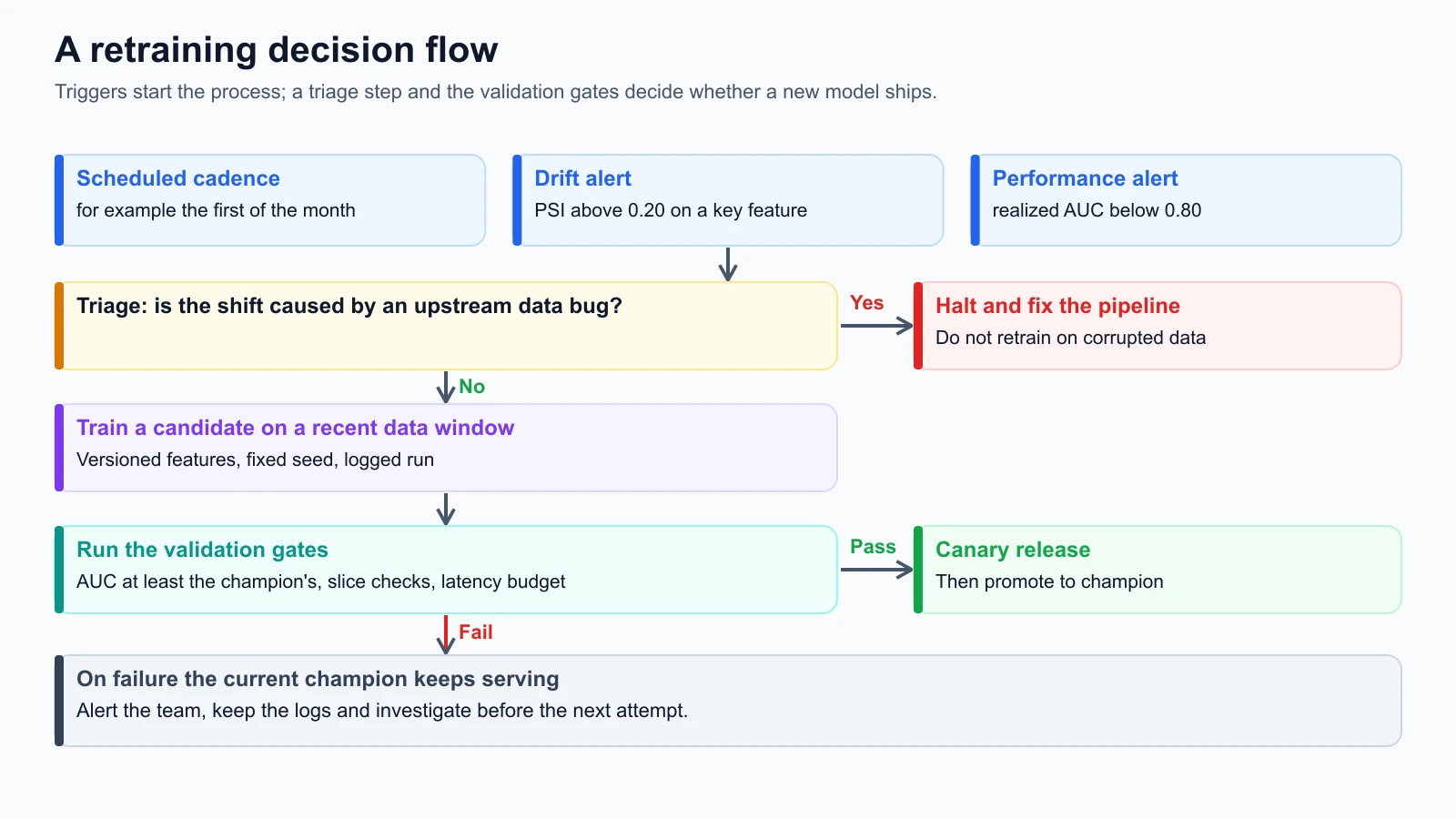
A disciplined automated retraining workflow follows five distinct phases:
Phase 1: Upstream root-cause triage (The critical gate)
Before writing a single training tensor, the pipeline must verify that the observed drift is not caused by an engineering defect. If an upstream ETL pipeline broke, a mobile app release renamed JSON keys, or an API gateway started dropping null values, halt the retraining pipeline immediately. Retraining on corrupted inputs produces a permanently crippled model. Data engineering must fix the upstream source first.
Phase 2: Training dataset windowing
When genuine drift occurs, how much historical data should you feed the retraining pipeline?
- Sliding window (e.g. last 90 days): Replaces old data with recent records. Ideal when fast-moving concept drift renders data from six months ago obsolete.
- Growing window (cumulative): Retains all historical records while appending new data. Ideal for highly cyclical or seasonal businesses where past patterns repeat predictably.
Phase 3: Automated training execution
The pipeline launches an isolated training job (e.g. on AWS SageMaker, Kubernetes, or Vertex AI) using versioned training scripts and tracked hyperparameters.
Phase 4: Validation and promotion gates
The newly trained candidate model must pass all rigorous evaluation gates described in evaluation and validation gates:
- Candidate AUC Champion AUC: The candidate must demonstrate superior or equal discrimination on a freshly collected holdout test cohort.
- Slicing and fairness checks: Performance must not degrade across vulnerable demographic or business customer tiers.
- Inference latency SLA: 99th percentile response time must remain within the 50ms budget.
Phase 5: Progressive canary rollout
If the candidate passes all validation gates, deploy it as a canary (routing 10% of live traffic). If operational error rates and prediction distributions remain stable over a 2-hour window, promote the candidate to 100% production traffic.
Production retraining runbook template
Every production MLOps system must maintain an executable Retraining Runbook in its project repository:
1# MLOps Retraining Runbook: [Model Name]
2
3* **System Name:** `staywell-churn-predictor`
4* **Current Champion Version:** `v1.4.2`
5* **On-Call Contact:** `#mlops-triage`
6
7## 1. Automated Triggers
8* **Cadence:** Scheduled monthly on the 1st at 02:00 UTC.
9* **Drift Threshold:** Key feature PSI >= 0.20 over rolling 7-day window.
10* **Performance Floor:** Realized 30-day AUC < 0.80.
11
12## 2. Pre-Flight Triage Checklist
13Before approving or debugging an automated retrain run, verify:
14- [ ] Upstream ETL pipelines completed with zero schema violations.
15- [ ] Feature missingness rates across all top 10 features remain < 0.5%.
16- [ ] No mobile client releases altered feature extraction logic in the past 14 days.
17
18## 3. Data Windowing Policy
19* **Training Window:** Sliding 90-day historical window.
20* **Test Cohort:** Holdout dataset from the most recent 14 calendar days.
21
22## 4. Promotion Gate Thresholds
23Candidate model must satisfy all conditions before production traffic routing:
24* Candidate Test AUC >= Champion Test AUC (or within 0.005 tolerance).
25* Brier calibration score <= 0.12.
26* P99 inference latency <= 50 milliseconds.
27* No individual demographic slice exhibits AUC degradation > 0.03.
28
29## 5. Rollback Procedure
30If the candidate model exhibits anomalous behavior during canary rollout:
311. Set Canary traffic weight to 0% via API gateway.
322. Route 100% of traffic back to Champion (`v1.4.2`).
333. File high-priority Jira ticket in `MLOPS` project with evaluation artifact logs.
Practical code: Production drift detector
Below is a self-contained, fully tested Python implementation of a production PopulationStabilityIndex drift detector. It supports both continuous numerical features (using quantile binning) and categorical features, includes epsilon smoothing to prevent zero-division errors, and flags drift severity tiers according to standard industry benchmarks.
drift_detector.py
1"""
2Production Drift Detector using Population Stability Index (PSI).
3
4Provides:
5- Quantile-based continuous feature binning
6- Categorical distribution drift analysis
7- Epsilon smoothing to prevent zero-division and logarithmic domain errors
8- Standardized drift classification (NO_DRIFT, MODERATE_DRIFT, SIGNIFICANT_DRIFT)
9"""
10
11from dataclasses import dataclass
12from typing import Dict, List, Any
13import math
14
15
16@dataclass(frozen=True)
17class DriftReport:
18    """Contains statistical results from a PSI evaluation."""
19    feature_name: str
20    psi_score: float
21    status: str  # "NO_DRIFT", "MODERATE_DRIFT", "SIGNIFICANT_DRIFT"
22    bucket_details: List[Dict[str, Any]]
23
24
25class PopulationStabilityIndex:
26    """Calculates PSI for continuous numerical and categorical distributions."""
27
28    def __init__(self, num_bins: int = 10, epsilon: float = 1e-4):
29        self.num_bins = num_bins
30        self.epsilon = epsilon
31
32    def calculate_continuous(
33        self,
34        reference: List[float],
35        target: List[float],
36        feature_name: str = "feature"
37    ) -> DriftReport:
38        """Calculate PSI on continuous numerical features using reference quantiles."""
39        if not reference or not target:
40            raise ValueError("Reference and target datasets must be non-empty")
41
42        ref_sorted = sorted(reference)
43        n_ref = len(ref_sorted)
44        n_target = len(target)
45
46        # Establish quantile bin edges based on reference distribution
47        bin_edges = []
48        for i in range(1, self.num_bins):
49            idx = int(round(i * (n_ref - 1) / self.num_bins))
50            bin_edges.append(ref_sorted[idx])
51
52        # Deduplicate edges to handle repeated or tied values
53        unique_edges = sorted(list(set(bin_edges)))
54
55        # Helper to assign data points into quantile buckets
56        def assign_bins(data: List[float]) -> List[int]:
57            counts = [0] * (len(unique_edges) + 1)
58            for val in data:
59                placed = False
60                for b_idx, edge in enumerate(unique_edges):
61                    if val <= edge:
62                        counts[b_idx] += 1
63                        placed = True
64                        break
65                if not placed:
66                    counts[-1] += 1
67            return counts
68
69        ref_counts = assign_bins(reference)
70        target_counts = assign_bins(target)
71
72        total_psi = 0.0
73        bucket_details = []
74
75        for b_idx in range(len(ref_counts)):
76            e_prop = ref_counts[b_idx] / n_ref
77            a_prop = target_counts[b_idx] / n_target
78
79            # Epsilon smoothing prevents division by zero or ln(0)
80            e_safe = max(e_prop, self.epsilon)
81            a_safe = max(a_prop, self.epsilon)
82
83            bucket_psi = (a_safe - e_safe) * math.log(a_safe / e_safe)
84            total_psi += bucket_psi
85
86            bucket_details.append({
87                "bucket_index": b_idx,
88                "expected_ratio": round(e_prop, 4),
89                "actual_ratio": round(a_prop, 4),
90                "psi_contribution": round(bucket_psi, 4)
91            })
92
93        total_psi = round(total_psi, 4)
94
95        if total_psi >= 0.20:
96            status = "SIGNIFICANT_DRIFT"
97        elif total_psi >= 0.10:
98            status = "MODERATE_DRIFT"
99        else:
100            status = "NO_DRIFT"
101
102        return DriftReport(
103            feature_name=feature_name,
104            psi_score=total_psi,
105            status=status,
106            bucket_details=bucket_details
107        )
108
109    def calculate_categorical(
110        self,
111        reference: List[str],
112        target: List[str],
113        feature_name: str = "feature"
114    ) -> DriftReport:
115        """Calculate PSI across discrete categorical frequencies."""
116        if not reference or not target:
117            raise ValueError("Reference and target datasets must be non-empty")
118
119        all_categories = sorted(list(set(reference) | set(target)))
120        n_ref = len(reference)
121        n_target = len(target)
122
123        ref_counts = {c: 0 for c in all_categories}
124        for c in reference:
125            ref_counts[c] += 1
126
127        target_counts = {c: 0 for c in all_categories}
128        for c in target:
129            target_counts[c] += 1
130
131        total_psi = 0.0
132        bucket_details = []
133
134        for c in all_categories:
135            e_prop = ref_counts[c] / n_ref
136            a_prop = target_counts[c] / n_target
137
138            e_safe = max(e_prop, self.epsilon)
139            a_safe = max(a_prop, self.epsilon)
140
141            bucket_psi = (a_safe - e_safe) * math.log(a_safe / e_safe)
142            total_psi += bucket_psi
143
144            bucket_details.append({
145                "category": c,
146                "expected_ratio": round(e_prop, 4),
147                "actual_ratio": round(a_prop, 4),
148                "psi_contribution": round(bucket_psi, 4)
149            })
150
151        total_psi = round(total_psi, 4)
152
153        if total_psi >= 0.20:
154            status = "SIGNIFICANT_DRIFT"
155        elif total_psi >= 0.10:
156            status = "MODERATE_DRIFT"
157        else:
158            status = "NO_DRIFT"
159
160        return DriftReport(
161            feature_name=feature_name,
162            psi_score=total_psi,
163            status=status,
164            bucket_details=bucket_details
165        )
Unit test suite validating synthetic distribution shifts
Here is the test suite that simulates synthetic baseline samples, moderate distribution shifts, severe mean shifts, and categorical mutations:
drift_detector_test.py
1import unittest
2import random
3from drift_detector import PopulationStabilityIndex
4
5
6class TestDriftDetector(unittest.TestCase):
7    def setUp(self):
8        self.psi = PopulationStabilityIndex(num_bins=10)
9        random.seed(42)
10
11    def test_identical_distributions_no_drift(self):
12        ref = [random.gauss(50.0, 10.0) for _ in range(1000)]
13        target = [random.gauss(50.0, 10.0) for _ in range(1000)]
14        report = self.psi.calculate_continuous(ref, target, "tenure_months")
15
16        self.assertLess(report.psi_score, 0.05)
17        self.assertEqual(report.status, "NO_DRIFT")
18
19    def test_moderate_continuous_drift(self):
20        ref = [random.gauss(50.0, 10.0) for _ in range(1000)]
21        # Slight mean shift from 50.0 to 53.5
22        target = [random.gauss(53.5, 10.0) for _ in range(1000)]
23        report = self.psi.calculate_continuous(ref, target, "tenure_months")
24
25        self.assertTrue(0.10 <= report.psi_score < 0.20)
26        self.assertEqual(report.status, "MODERATE_DRIFT")
27
28    def test_significant_continuous_drift(self):
29        ref = [random.gauss(50.0, 10.0) for _ in range(1000)]
30        # Major mean shift from 50.0 to 65.0
31        target = [random.gauss(65.0, 10.0) for _ in range(1000)]
32        report = self.psi.calculate_continuous(ref, target, "tenure_months")
33
34        self.assertGreaterEqual(report.psi_score, 0.20)
35        self.assertEqual(report.status, "SIGNIFICANT_DRIFT")
36
37    def test_categorical_drift(self):
38        ref = ["month-to-month"] * 500 + ["one-year"] * 300 + ["two-year"] * 200
39        # Target experiences sharp drop in two-year contracts
40        target = ["month-to-month"] * 850 + ["one-year"] * 100 + ["two-year"] * 50
41
42        report = self.psi.calculate_categorical(ref, target, "contract_type")
43        self.assertGreaterEqual(report.psi_score, 0.20)
44        self.assertEqual(report.status, "SIGNIFICANT_DRIFT")
45
46    def test_unseen_category_handled_gracefully(self):
47        ref = ["month-to-month"] * 700 + ["one-year"] * 300
48        # Target introduces a brand new category not present in reference
49        target = ["month-to-month"] * 500 + ["one-year"] * 200 + ["three-year"] * 300
50
51        report = self.psi.calculate_categorical(ref, target, "contract_type")
52        self.assertGreaterEqual(report.psi_score, 0.20)
53        self.assertEqual(report.status, "SIGNIFICANT_DRIFT")
54
55
56if __name__ == "__main__":
57    unittest.main()
Save both files in the same folder and run the tests from that folder:
1python3 -m unittest discover -p '*_test.py'Mistakes beginners make
1. Retraining immediately without root-cause triage
When drift alerts fire, engineers often launch automated retraining jobs immediately. If the drift was caused by an upstream software bug (such as an ETL failure that started writing zeros into the support_tickets column), retraining on that corrupted data bakes the bug directly into the model weights, crippling model accuracy permanently.
Fix: Establish a mandatory root-cause triage gate. Always verify upstream pipeline health, feature null rates, and schema contracts before initiating any retraining workflow.
2. Relying strictly on hypothesis test p-values at scale
Developers frequently use two-sample Kolmogorov-Smirnov (KS) tests and trigger automated retrain alarms whenever the p-value drops below 0.05. In production environments processing 500,000 inference requests daily, tiny and harmless shifts produce near-zero p-values, creating perpetual false alarms.
Fix: Use effect size metrics like Population Stability Index (PSI) or Wasserstein distance that measure the practical magnitude of the shift rather than statistical significance alone.
3. Deploying retrained models without validation gates
Teams often configure automated CI/CD runners to automatically deploy retrained models to production as soon as the training script finishes. If recent data was noisy, contaminated, or subject to sudden market anomalies, the retrained model can easily perform worse than the champion model it replaces.
Fix: Enforce automated validation gates (as described in evaluation and validation gates). A newly retrained candidate must outperform the incumbent champion on holdout test cohorts, pass demographic fairness slices, and meet latency SLAs before receiving production traffic.
4. Keeping stale historical data indefinitely
When retraining models, teams often train on their entire cumulative multi-year database. If the business has experienced structural concept drift (such as changes in consumer habits or competitor pricing), ancient training data from two years ago pulls model weights in the wrong direction.
Fix: Adopt a sliding window data curation strategy (such as training on the most recent 90 to 180 days). Periodically test whether dropping historical data older than six months improves out-of-time validation metrics.
Recap and try it yourself
In this lesson, we explored how to detect statistical decay and maintain production model performance:
- Classify the drift mode: Distinguish between covariate shift ( changes), concept drift ( changes), and prior probability shift ( changes) to choose the correct remediation.
- Quantify divergence with PSI: Use the Population Stability Index to measure practical distribution shifts against standard industry thresholds ( stable, to moderate, significant).
- Avoid the sample size trap: Rely on effect size metrics (PSI) rather than p-values on high-volume production datasets.
- Enforce triage before retraining: Verify that observed drift is not caused by upstream ETL bugs or schema corruption before retraining.
- Gate all retrained candidates: Never promote a retrained model without verifying that candidate metrics surpass the champion on holdout cohorts.
Hands-on exercises
- Simulate a variance shift:
Using the
PopulationStabilityIndexclass from our practical code, generate a reference distribution of 1,000 samples with mean 50.0 and standard deviation 10.0. Generate a target distribution with the exact same mean (50.0) but double the standard deviation (20.0). Calculate the continuous PSI score. Does a pure variance shift trigger significant drift? - Draft a retraining incident plan: Suppose StayWell's marketing team introduces a "Free Tablet with 2-Year Plan" promotion. Churn among 2-year contract holders jumps from 2% to 25% because users cancel after receiving the hardware. Draft an entry in your Retraining Runbook outlining whether this represents data drift or concept drift, and specify what new features the team should create.
- Implement multiple testing correction: When evaluating PSI across 45 model features simultaneously, random sampling noise can cause at least one feature to exhibit moderate drift by chance. Modify the drift reporter to evaluate an aggregate drift score across all features, requiring at least two critical features to breach the 0.20 threshold before flagging an automated retrain alert.